Download
1 / 43
430 likes | 555 Views
LOW FREQUENCY INTERFEROMETRY. Roberto Francesco Pizzo, ASTRON ( The Netherlands ). ERIS 2011, 2011 September 8. OUTLINE Definition History What is to be investigated? The end and the new beginning of LF interferometry Ionosphere RFI A-team removal Large FOV all-sky imaging

E N D
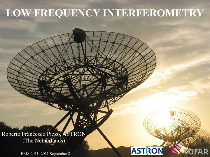
LOW FREQUENCY INTERFEROMETRY Roberto Francesco Pizzo, ASTRON (The Netherlands) ERIS 2011, 2011 September 8
OUTLINE • Definition • History • What is to be investigated? • The end and the new beginning of LF interferometry • Ionosphere • RFI • A-team removal • Large FOV all-sky imaging • Polarization issues
WHAT IS LOW FREQUENCY? • The general definition of low frequency is (Wikipedia): “Low frequency or low freq or LF refers to radio frequencies (RF) in the range of 30 kHz–300 kHz” • • NOT THE GENERAL DEFINITION USED BY ASTRONOMERS • LF radio astronomy ranges between 3 - 400 MHz • Ground-based instrument have 10 MHz as a lower limit due to reflection of the signal by the ionosphere.
HISTORY OF LOW FREQUENCY INTERFEROMETRY (I) • 1931-35 - Jansky: Birth of Radio astronomy, • discovery of Galactic emission • ν ~ 15 – 30 MHz • 1935-45 – Reber: discovery of • non-thermal • emission 160 MHz, resolution=12o
HISTORY OF LOW FREQUENCY INTERFEROMETRY (II) • 1946 – Ryle: construction of the first 2-element interferometer • 1955 – Kraus et al.: first all sky survey (ν = 80 MHz) • Burke et al.: discovery of the first planetary radio emission (ν = 10 - 100 MHz) • 1958-88 – Erickson: building of the Clarke Lake TPT (ν = 100 - 1400 MHz) • 1962 – Bennet: completion of the first 3C catalogue (ν = 160 MHz) • 1963 – Hazard Schmidt Sandage: discovery of the first quasar (ν = 178 MHz) • 1967: first VLBI fringes (ν = 20 - 1400 MHz) • 1968 – Bell: discovery of the first pulsar (ν = 81 MHz) • 1975-90: completion of the Cambridge 8C catalogue
LOW FREQUENCY RADIO INTERFEROMETERS LOFAR (NL – Europe) 10 - 240 MHz WSRT (NL) 270 – 390 MHz (but also 115-180 MHz) VLA (New Mexico - US) 300 – 350 MHz (later also 74 MHz) GMRT (India) 150, 232, 325 MHz LWA (New Mexico – US) 10 – 80 MHz MWA (AUS) 80 – 300 MHz SKA < 70 --- 30000 MHz (?) Modern sensitive interferometers Future arrays = with dipoles
LOW FREQUENCY RADIO INTERFEROMETERS LOFAR (NL – Europe) 10 - 240 MHz WSRT (NL) 270 – 390 MHz (but also 115-180 MHz) VLA (New Mexico - US) 300 – 350 MHz (later also 74 MHz) GMRT (India) 150, 232, 325 MHz LWA (New Mexico – US) 10 – 80 MHz MWA (AUS) 80 – 300 MHz SKA < 70 --- 30000 MHz (?) Modern sensitive interferometers Future arrays A PERFECT TIME TO DO LF RADIOASTRONOMY !!! = with dipoles
LOW FREQUENCY SKY: WHAT IS TO BE INVESTIGATED? • Thermal emission (Free-free, Bremsstrahlung): • Best observed at ν> 1 GHz • Due to deflection of electrons by ions • Depends on gas temperature • Synchrotron emission: • Best detected at ν < 1 GHz ( ) • Particles spiraling around B lines • Polarized • Intensity depends on energy of e and strength of B
LOW FREQUENCY SKY: WHAT IS TO BE INVESTIGATED? Cas A, 76 MHz • Radio recombination lines: • Largely observed toward the Galactic plane and discrete sources. Detected n absorption below 150 MHz • They provide a diagnostic of the physical condition of the poorly known cold ISM (temperature, density, level of ionozation, abundance ratios, etc… Cas A, 26 MHz Stepkin et al. 2007
SCIENCE UNIQUE TO LF RADIOASTRONOMY Epoch of Reionization (highly redshifted 21 cm line) Early structure formation (high z RG) Large scale structure formation (diffuse emission) Wide field mapping Large surveys Serendipity: exploration of the unknown ISM, HII regions, SNR, pulsars Galaxy evolution Transient searches Ionospheric studies Solar burst studies
LIMITS OF LF RADIO ASTRONOMY: IONOSPHERIC BARRIER • Spatial resolution increases with the antenna interferometer baseline: • First long wavelength interferometers had very poor spatial resolution • Large arrays of mechanically mounted parabolas are very costly! • Low frequency instruments needed limited aperture due to the ionosphere (B < 5 km for ν < 100 MHz)
ABANDONING LF RADIO ASTRONOMY • Confusion: it manifests in several fundamentally different ways, including main-beam, side-lobe, and classical confusion sensitivity degraded by • Imaging of large fields of view posed enormous computing problems • Removal of RFI (radio frequency interferences) was challenging • Astronomers pushed for better resolution and continued their work at high frequencies. = 10’, σ = 30 mJy/beam = 1’, σ = 3 mJy/beam
WHY NEW INTEREST FOR LF RADIOASTRONOMY ? • We can use phased arrays: antennas in which the relative phases of the respective signals feeding the antennas are varied in such a way that the effective radiation pattern of the array is reinforced in a desired direction and suppressed in undesired directions • Enormous flexibility: electronic beamformingand ‘software telescope’ • Advantages: a) replacement of mechanical beam forming by electronic signal processing • b) low frequency telescopes become economically affordable • c) multiple and independent beams can be formed at a time Receiver Physical delay Receiving array Parabolic reflector Correlator Output
WHY NEW INTEREST FOR LF RADIOASTRONOMY ? • because with the current capabilities of radio interferometers, we can … • achieve 1000x better sensitivity, • with an appropriate image quality (>104 dynamic range), • at a resolution of 0.25-1.0 arcsecover the whole sky, • do it in full polarization and do spectroscopy at z = 10, • record down to 5 ns resolution, • in somewhat difficult RFIconditions, • and do this for many users simultaneously.
NOT EN EASY TASK… • The lower the observing frequency, the larger is the field of view (FOV) of your telescope LF observations require imaging and (self-)calibration of the whole sky. • E.g. @ 100 MHz • HPBW ~ 1.3 λ / D ~ 10o for D = 25 m (WSRT, VLA) • A-team: CasA, CygA ~ 10.000 Jy • VirA, TauA ~ 1.000 Jy • Sun ~ > 10.000 – 1000,000 Jy • Even far from the field center, the (relatively) high distant sidelobe levels of the primary beam (‘only’ -30 to -40 db) keeps these sources very bright, giving rise to significant sidelobes in the final images.
THE A-TEAM around A2255 @ 115 MHz (WSRT) Tau A Sun Cas A Cas A Cyg A Vir A A2255
THE A-TEAM around A2255 @ 115 MHz (WSRT) Tau A Sun Cas A Cas A This effect is even more dramatic for dipole arrays, which ‘see’ the entire sky down to the horizon Cyg A Vir A A2255
THE CHALLENGES OF LF RADIO IMAGING • The phase stability of the received signal is an important factor at whatever frequency we are working. Two main factors contribute to corrupt phase stability: • Instrument (geometry + electronics) • Atmosphere = troposphere + ionosphere • TROPOSPHERE: 0 - 10 km • IONOSPHERE: 100 – 1000 km • The ionospheric disturbances become progressively more important at low frequencies, while the tropospheric effect become negligible • LOOKING AT THE IONOSPHERE IS CRUCIAL
IONOSPHERE Portion of the upper atmosphere, which extends from about 100 to 1000 km above the Earth, where ions and electrons are present in quantities sufficient to affect the propagation of electromagnetic waves • During the day, molecules bombarded by solar X-ray and UV radiation ‘ions’ are produced. Recombination at night. • Degree of ionization varies greatly with time (sunspot cycle, seasonally and diurnally) and geographical location (polar, mid-latitude, and equatorial regions) • Refractive index: • where • When ν < νp, wave reflection • (ν < 10 MHz) solar maximum solar minimum
VERTICAL TOTAL ELECTRON CONTENT • Total number of electrons present along a path between two points, with units of electrons per square meter, where 1016 electrons/m² = 1 TEC unit (TECU) • Data obtained through GPS satellites (movie courtesy of A. Burns, T. Killeen and W. Wang at the University of Michigan)
IONOSPHERIC WEDGE MODEL IONOSPHERE position • Differential delay due to ionospheric density gradient • i.e. depends on baseline length, not station or ionosphere position
FOR LONG BASELINES… IONOSPHERE > 5 km < 5 km coherence preserved lost coherence • Over long distances, the ionospheric regions crossed by the signal have very different properties we loose the coherence of the signal – gradient approach fails (also for large separations in the sky) • Minimum allowed baseline size given by the size scale of the Traveling IonosphericDisturbancies (TDIs). For ν < 100 MHz, coherence of the signal preserved for baseline length < 5 km
NON ISOPLANATICITY • At low frequencies, phase fluctuations are dominated by ionospheric effect also because primary beam is larger than the coherence length of the ionosphere • the primary beam illuminates a portion of sky in which the ionosphere behaves • as a variable refractive medium. The electromagnetic wave propagates through • this wedge with different velocities, therefore with variable refractive indices • Area in which the wavefront is still plane: isoplanatic patch • Variations of the ionospheric phase over the field of view are referred to as non isoplanaticity
(SELF-)CALIBRATION AT LOW FREQUENCIES • High dynamic range imaging seriously limited by the stability of the ionosphere • Selfcal algorithm minimizes the differences between model and data by applying an average time-dependent correction to the field not ok when the FOV is large and samples various isoplanatic patches • Direction dependent calibration must be applied to the data, by removing the problematic off-axis sources together with their calibration corrections (Cotton et al. 2004, Intema 2009) • • PEELING A773, WSRT @ 325 MHz
AN EXAMPLE: A2255 with WSRT • Presence of spiky pattern surrounding the brightest off-axis sources . Pattern due to the instantaneous fan beam response of WSRT, rotating clockwise from position angle +90o to +270o in the 12h synthesis No peeling applied Peeling applied FWHM ~ 1’ σ ~0.1 mJy/beam λ= 25 cm
BANDWIDTH SMEARING • Averaging the visibilities over finite BW results in chromatic aberration, which worsens with distance from the phase center radial smearing • Does not affect the target source, but it must be corrected to properly deconvolvethe images • Effects can be parametrized by the product of the fractional bandwith and the source offset in synthesized beamwidths • increases with angular resolution and radial distance • when of the order of unity, chromatic aberration becomes an issue: • Solution: observe in spectral line continuous mode (which also helps the RFI excision) point source at 7’ from the field center at 20 cm, VLA Courtesy of E. Orru’
RADIO FREQUENCY INTERFERENCE (RFI) • One of the most serious problems of low frequency interferometry • Two origins: • a) natural: lighting static during summer time, dust particles attracting charged particles in the proximity of the antennas. • Solar bursts (night time preferred), geo-magnetic storms, ionospheric scintillations • b) man-made: have various origin, residing in the electronic equipment present in the • antennas themselves. At meter wavelengths, significant contribution comes from • - TV 50 – 700 MHz • - FM radio 88 – 108 MHz • - Digital audio broadcast 174 – 230 MHz, Europe • - Satellites • … • RFI measurement and monitoring are essential to ensure a good quality of radio data
RFI in THE NETHERLANDS (similar to all EU) Max observed RFI signal level ~ - 110 dbWm-2Hz-1 ~ 1015 Jy (at 169 MHz) Antenna sky noise level ~ - 201 dbWm-2Hz-1 ~ 106Jy(at 150 MHz) CasA/CygA ~ - 219 dbWm-2Hz-1 ~ 104 Jy (at 150 MHz)
RFI MITIGATION • Phased arrays are particularly interesting for their capabilities to do interference suppression • If the same interfering signal is received by several antenna elements, then by properly phasing and combining the antennas, that signal can be nulled. • In practice, there are several complications: there are many interfering signals; the signals nor their directions are known; they are often time-varying; and signal nulling will also disturb the reception of the sky signals. • It can be applied in two different stages: (i) pre-correlation and (ii) post-correlation • Very powerful, as it is applied to full resolution data. Several methods from signal processing to handle this step, eg spatial filtering: at station level, beamshape modified such that interferer is nulled; at central level, signals combined to null any residual RFI • Manual flagging, but also fringe fitting (Athreya 2009) and post-correlation spatial filtering are possible.
AN AD HOC FLAGGERFOR LOFAR DATA • AOFlagger (RFIconsole) is based on the ‘SumThreshold’ method, which detects series of samples with higher values than expected • Analysis done iteratively for the entire observation, per sub band, per baseline • Method is very accurate. The algorithm finds RFI invisible by eye on full scale time-frequency diagrams Time-frequency before flagging Time-frequency after flagging 156 MHz, 1.8% data flagged Amplitude plot before flagging Amplitude plot after flagging courtesy of Andre’ Offringa
BRIGHT SOURCES REMOVAL – THE A-TEAM • The presence of very bright sources in the low-frequency sky (Cyg A, CasA, VirA, TauA, HerA + Sun), combined with the large beam size of LF arrays (LOFAR ~ 10o at ν = 80 MHz) seriously limits the dynamic ranges needed for extragalactic surveys (~ 10.000) • Three main methods are being explored to remove the A-team sources: • direction dependent calibration (peeling); good source model needed and no compression applicable; computationally very intensive; • multi beam approach: A-team and target source observed in different beams; phase-rotate the A-team sources uv-data towards the target field and directly subtract them after re-normalizing by the beam. If cross-contamination between A-team sources datasets plays a role, solve linear systems well described by the measurement equation; • demixing: based on the assumption that the interfering sources are far from the field center, so their fringe rate is high with respect to the target field (it can work with highly averaged data)
EXAMPLE OF DEMIXING (HydA) VLA, 74 MHz Courtesy of R. van Weeren Hydra A, after demixing -12 declination (!) 50 MHz 1 SB, 127o (!!) from pointing center (Hydra A)
WIDE FIELD IMAGING • The sky brightness is obtained as a 2-D Fourier inversion of the visibilities. True if we assume: • all the visibilities measurements lie in a plane (w term can be neglected) • FOV limited to a small angular region • There are two methods of wide field imaging: • imaging the field in different facets or polyhedron corresponding to different positions on the celestial sphere by phase rotating the uv data for each one of those. • W-projection using a w-dependent convolution function in the gridding step to retrieve an undistorted image after a simple 2D fast Fourier transform
WIDE FIELD IMAGING (FACETTING) • Full pixellation is computationally prohibitive! • Use NVSS or WENSS to set outliers • No need to image empty space • (unless you are doing a survey) • Loss of potential science Fly’s eye 4 degrees VLA A arrary requires 10.000 pixels!!! Outliers
WIDE FIELD IMAGING (W-PROJECTION) • Simulated observation at 74 MHz with VLA C configuration • Sources brighter than 2 Jy taken from WENNS within 12o from phase center • W-projection an order of magnitude faster than facets • Distortion of sources far from field center for case a) and b) • c) much better than b) in case of great sensitivities Cornwell et al. 2008
FUTURE OF WIDE FIELD IMAGING: A-PROJECTION • In situations in which time and frequency independence are not satisfied, a new imaging technique must be used. For LOFAR, antenna gains are direction, time, and frequency dependent. Faceting still holds, but deconvolution scheme is complicated A-projection, where DDE and non complanarity of the array are corrected in a way similar to the w-projection algorithm. • Vary in terms of computing efficiency (faster than facet-based algorithms by an order of magnitude), and it can potentially take all DDE into account in the deconvolution steps. Currently being tested on both simulated and real LOFAR data.
POLARIZATION ASPECTES AT LOW FREQUENCY
THE POTENTIAL • New frontier ! • Great diagnostic value to characterize the properties of emitting source and media crossed by its polarized signal (Faraday rotation): • ISM, IGM • Ionosphere (time variable!) observer Magnetized plasma Faraday rotation Linearly Polarized radiation Magnetic field B source
TECHNICAL ASPECTS AT LOW FREQUENCY • Propagation and instrumentation lead to various depolarization effects: • I. beam use longer baselines • (WSRT 3 km, VLA-GMRT 30 km, LOFAR ~ 100 – 1000 km) • II. bandwidthuse multi-channel backends • III. depthseparate Faraday (think/thick) layers in RM-space
BEAM DEPOLARIZATION • when the magnetic field is tangled on scales smaller than the resolution of the observations, the original signal depolarizes inside the observingbeam • EXAMPLES: • ISM RM-gradient of 1 rad m -2 per degree translates at 50 MHz to a rotation of the polarization vector of 34o/arcmin • • LOFAR-100 km has no problem • Source RM-gradient of 1 rad m-2 per arcmin translates at 50 MHz into a rotation of the polarization vector of 34o/arcsec • • 1000 km baselines are needed
BANDWIDTH DEPOLARIZATION • observations are carried out in a frequency band with a particular bandwidth Δν • This corresponds to • 0.03 o/kHz at 150 MHz for a RM = 10 rad m-2 • 0.08 o/kHz at 50 MHz “ • 3.8 o/kHz at 30 MHz “ • kHz resolution achieved by LOFAR, for which RM synthesis becomes an obvious tool to adopt to process polarimetric data
RM SYNTHESIS ON PSR J0218+4232 • 800 frequency channels • 25σ detection • RM = -61 rad m-2 3C66 Courtesy of Martin Bell
SUMMARY • Low frequency interferometry is a powerful tool to answer several interesting question about the history of the universe • Several challenges have to be faced when trying to process low frequency data • Various techniques have been recently develop to deal with issues related to the ionosphere, large FOV, RFI in low frequency data • Low frequency interferometry is undergoing a new golden age, which will surely lead to some important discoveries • It is a perfect time to do LF radio astronomy!