Download

1 / 29
320 likes | 452 Views
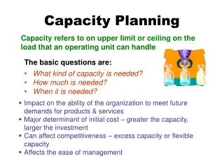
Capacity Planning. Capacity. Capacity ( I ): is the upper limit on the load that an operating unit can handle. Capacity ( II ): the upper limit of the quantity of a product (or product group) that an operating unit can produce (= the maximum level of output)

E N D
Capacity • Capacity (I): is the upper limit on the load that an operating unit can handle. • Capacity (II): the upper limit of the quantity of a product (or product group) that an operating unit can produce (= the maximum level of output) • Capacity (III): the amount of resource inputs available relative to output requirements at a particular time
Capacity • Design capacity • maximum output rate or service capacity an operation, process, or facility is designed for • = maximum obtainable output • = best operating level • Effective capacity • Design capacity minus allowances such as personal time, maintenance, and scrap(leftover) • Actual output = Capacity used • rate of output actually achieved. It cannot exceed effective capacity.
Capacity Efficiency and Capacity Utilization Actual output Efficiency = Effective capacity Actual output Utilization = Design capacity
Determinants of Effective Capacity • Facilities,layout • Product and service factors • Process factors • Human factors • Policy (shifts, overtime) • Operational factors • Supply chain factors • External factors
Capacity Cushion • level of capacityin excess of the average utilization rate or level of capacity in excess of the expected demand. • Capacity cushion = (designed capacity / capacity used) – 1 • Sources of Uncertainty • Manufacturing • Customer delivery • Supplier performance • Changes in demand
The „Make or Buy” problem • Available capacity • Expertise • Quality considerations • Nature of demand • Cost • Risk
Developing Capacity Alternatives • Design flexibility into systems • Take stage of life cycle into account (complementary product) • Take a “big picture” approach to capacity changes • Prepare to deal with capacity “chunks” • Attempt to smooth out capacity requirements • Identify the optimal operating level
Adapting capacity to demand through changes in workforce DEMAND PRODUCTION RATE (CAPACITY)
Adaptation with inventory DEMAND Inventory reduction Inventory accumulation CAPACITY
Adaptation with subcontracting DEMAND SUBCONTRACTING PRODUCTION (CAPACITY)
Adaptation with complementary product PRODUCTION (CAPACITY) DEMAND DEMAND PRODUCTION (CAPACITY)
Minimum average cost per unit Average cost per unit Minimumcost 0 Rate of output Economies of Scale • Economies of scale • If the output rate is less than the optimal level, increasing output rate results in decreasing average unit costs • Diseconomies of scale • If the output rate is more than the optimal level, increasing the output rate results in increasing average unit costs Production units have an optimal rate of output for minimal cost.
Evaluating Alternatives II. Minimum cost & optimal operating rate are functions of size of production unit. Small plant Medium plant Average cost per unit Large plant 0 Output rate
Designed capacity in calendar time CD= N ∙ sn ∙ sh ∙ mn ∙ 60 (mins / planning period) • CD= designed capacity (mins / planning period) • N = number of calendar days in the planning period (365) • sn= maximumnumber of shifts in a day (= 3 if dayshift + swing shift + nightshift) • sh= number of hours in a shift (in a 3 shifts system, it is 8 per shift) • mn= number of homogenous machine groups
Designed capacity,with given work schedule C’D= N ∙ sn ∙ sh∙ mn ∙ 60 (mins / planning period) • C’D= designed capacity (mins / planning period) • N = number of working days in the planning period (≈ 250 wdays/yr) • sn= number of shifts in a day (= 3 if dayshift + swing shift + nightshift) • sh= number of hours in a shift (in a 3 shifts system, it is 8) • mn= number of homogenous machine groups
Effective capacityinworkingminutes CE= CD- tallowances (mins / planning period) CD= designed capacity tallowances= allowances such as personal time, maintenance, and scrap (mins / planning period) b = ∙ CE b = expected capacity(that we use in product mix decisions) CE= effective capacity = performance percentage
Exercise 1. A company produces a product in 2 shifts pattern and 250 days in a given year. Two machines are available in the workstation. The maintenance needs 8 hours in a month. The performance rate in the first shift is 90%, in the second shift 80%. Each product needs 25 minutes to be finished. • a) Determine the designed capacity for one year. • b) Determine the effective capacity for one year. • c) Determine the expected capacity for one year. • d) Determine the number of products we can produce. • e) Determine the utilization and efficiency if the actual output is 15 800 pieces. • d) Determine capacity cushion.
Exercise 2. Set up the product-resource matrix using the following data! • RP coefficients: a11: 10, a22: 20, a23: 30, a34: 10 • The planning period is 4 weeks (there are no holidays in it, and no work on weekends) • Work schedule: • R1 and R2: 2 shifts, each is 8 hour long • R3: 3 shifts • Homogenous machines: • 1 for R1 • 2 for R2 • 1 for R3 • Maintenance time: only for R3: 5 hrs/week • Performance rate: • 90% for R1 and R3 • 80% for R2
Solution (bi) • Ri = N ∙ sn ∙ sh ∙ mn ∙ 60∙ • N=(number of weeks) ∙ (working days per week) • R1 = 4 weeks∙ 5 working days∙ 2 shifts∙ 8 hours per shift∙ 60 minutes per hour∙ 1 homogenous machine∙ 0,9 performance = = 4 ∙ 5 ∙ 2 ∙ 8 ∙ 60 ∙ 1 ∙ 0,9 = 17 280 minutes per planning period • R2 = 4 ∙ 5 ∙ 2 ∙ 8 ∙ 60 ∙ 2 ∙ 0,8 = 30 720 mins • R3 = (4 ∙ 5 ∙ 3 ∙ 8 ∙ 60 ∙ 1 – 5 hrs per week∙ 60 minutes ∙ 4 weeks) ∙ 0,9= (28 800 – 1200 ) ∙ 0,9= 24 840 mins
Exercise 1.2 • Complete the corporate system matrix with the following marketing data: • There are long term contract to produce at least: • 50 P1 • 100 P2 • 120 P3 • 50 P4 • Forecasts says the upper limit of the market is: • 10 000 units for P1 • 1 200 for P2 • 1 000 for P3 • 2 000 for P4 • Unit prices: P1=100, P2=200, P3=330, P4=100 • Variable costs: R1=5/min, R2=8/min, R3=11/min
What is the optimal product mix to maximize revenues? • P1= 17 280 / 10 = 1728 < 10 000 • P2= 100 • P3= (30 720-100∙20-)/30= 957<MAX • P2: 200/20=10 • P3: 330/30=11 • P4=24 840/10=2484>2000
What if we want to maximize profit? • The only difference is in P4 because of its negative contribution margin. • P4=50
Solution Revenue max. • P1=333 • P2=400 • P3=400 • P4=200 • P5=1000 Contribution max. • P1=333 • P2=500 • P3=250 • P4=100 • P5=1000