Download

1 / 23
230 likes | 238 Views
Parametric Approaches to Welfare Measurement. Background.

E N D
Background • Up until now our examination of welfare has been essentially non-parametric in a statistical sense, we have not specified or estimated the parametric structure of the size distributions of income rather we have compared distributions via the empirical distributions functions directly. • When we know the parametric structure of distributions some welfare implications can be inferred directly. (e.g. x~N(10,10), y~N(10+ε,10) → y FOD x and x~N(10,10), y~N(10,10-ε) → y SOD x). (There also exist explicit formulae for many of the inequality indices). • There is an old and more recent literature which considers specifying and estimating size distributions of income and making such comparisons.
[A] Processes that Generate Log Normal Y under CLT arguments. • Letting Y=ln(y=Income) yields what is called the Law of Proportionate Effects. Used most frequently in a time series context from the notion that yt=yt-1(1+et) where et is considered i.i.d. and E(et) = growth rate with V(et) small relative to 1. • Gibrats Law (Gibrat (1930),(1931)): Yti = μi + Yt-1i + Uti implies for process of life length T, Y ~ N(μT,σ2T) i.e. y is non-stationary • Kalecki’s modification (Kalecki(1945)): Yti = μi + βiYt-1i + Uti where |βi| < 1; a stationary version of Gibrat’s Law. Y ~ N(μ/(1-β),σ2/(1-β2)).
Models of the Size Distribution of Income (Y=ln(per capita income) • [B] Processes that generate “Pareto” type distributions under CLT arguments (Pareto (1897)) • Gabaix (1999); Y(i,t)= μ(i) + Y(i,t-1) + u(i,t) (with Y(i,t) bounded from below) • Champernowne (1953) Markov Chain Process where f(yt)=Mf(yt-1) with M a lower triangular transition matrix • Double Pareto (Reed(2001)) Y(i,t)= μ(i) + Y(i,t) + u(i,t) (“t” governed by an exponential process)
Models of the Size Distribution of Income (Y=ln(per capita income) • [C] Ad Hoc Parametric Generalizations Mandelbrot(1960) Singh and Maddala (1976) McDonald (1984) Houthakker (2002)
Tests for verifying the model specification. • Pearson’s Goodness of Fit Test. Partition the range of x into K mutually exclusive and exhaustive intervals then for a sample of size n let Ei be the number of observations expected in the i’th interval and let Oi be the number of observations actually observed in the i’th interval i=1,..,K then ΣKi=1(Oi-Ei)2/Ei ~ χ2(K-1-h) where h is the number of estimated parameters needed to calculate the Ei. • Kolmogorov- Smirnov Test (see previous lecture) • Hall Yatchew Expected Squared Difference Test.(see previous lecture).
Poverty rates under Gibrat’s Law • For an absolute poverty line x* • limT->∞ Φ([(ln(x*/x0)-T(μ+0.5σ2))/(σ√T)]) • Growth exceeding -0.5σ2 implies a poverty rate of 0 in the limit, for growth less than -0.5σ2 the poverty rate would be 1. • For a relative poverty line (0.6 of median income) the poverty rate would be Φ([ln(0.6)/(σ√T)]) which increases with time reaching .5 at infinity.
Poverty and Inequality Under Pareto’s Law • Poverty and inequality measures would be constant over time • The Gini for a Pareto distribution is 1/(2θ-1) which is 1 when the shape coefficient is one because in this case the Pareto distribution has no moments or an infinite mean. • If the poverty frontier is a real lower boundary below which no-one is allowed to fall, the income distribution would end up as Pareto – hence a very strong test of the efficacy of such a frontier.
The Gini under Gibrat’s Law • Gini may be written as: 2F(exp(ln(x0)+T(μ+0.5σ2))| exp(ln(x0)+T(μ+0.5σ2)),Tσ2 ) – 1 where F(z | θ, γ ) is the log normal distribution function with mean and variance θ, γ respectively • This will tend to zero as T => ∞ when μ < -0.5σ2 and will tend to 1 otherwise, note particularly for zero growth Gini will tend to 1.
Polarization and Mixtures • If we think of societal income distributions as mixtures then we can analyze the progress of rich and poor groups as distinct entities. • Use the Trapezoidal Index as a measure of relative poverty. • 0.5(wpfp(xmp)+(1-wp)fr(xmr))(xmr-xmp)
Parametric Approaches to Mixture Distributions. • To facilitate modeling one can fit distributions to the data and track the fitted sub distributions. • To illustrate these issues data on per capita GDP for 47 African countries together with their populations were drawn from the World Bank African Development Indicators CD-ROM for the years 1985, 1990, 1995, 2000, 2005 were used
Comments • Growth rate in the mean and variance greater in the un-weighted sample than in the weighted sample • Much more evidence for Log normality than for Pareto.