Download
1 / 12
120 likes | 124 Views
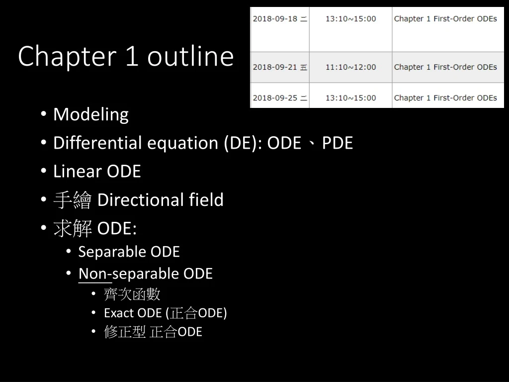
Chapter 1 outline. Modeling Differential equation (DE): ODE 、 PDE Linear ODE 手 繪 Directional field 求解 ODE: Separable ODE Non- separable ODE 齊次函數 Exact ODE ( 正合 ODE) 修正型 正 合 ODE. Mathematical Models.

E N D
Chapter 1outline • Modeling • Differential equation (DE): ODE、PDE • Linear ODE • 手繪 Directional field • 求解 ODE: • Separable ODE • Non-separable ODE • 齊次函數 • Exact ODE (正合ODE) • 修正型 正合ODE
Mathematical Models • If we want to solve an engineering problem (usually of a physical nature), we first have to formulate the problem as a mathematical expression in terms of variables, functions, equations, and so forth. • Such an expression is known as a mathematical model.
(Mathematical) Modeling • The process of (1) setting up a model, (2) solving it mathematically, and (3) interpreting the result in physical or other terms; is called mathematical modeling, or, briefly, modeling. • All math models can be solved (obtaining solutions) one way or the others. However this mathematical solution is not necessarily a solution to the engineering (physical) problem.
Physical System Mathematical Model Mathematical Solution Physical Interpretation
Differential Equations 微分方程 (DE) • Since many physical concepts, such as velocity and acceleration, are derivatives, a model is very often an equation containing derivatives of an unknown function. • Such a model is called a differential equation.
Fig. 1. Some applications of differential equations Newton’s second law of motion
Concept of a solution • Given an simple ODE below, the solution y(x) is a function of x, whose first derivative with respect to x is cos x.
Classification of DEs • ODE: Note that an ODE involves a function with one independent variable (自變數) only. • PDE: For DEs with two or more independent variables, we called them partial differential equations, or PDEs.
Concept of a solution • Given an simple ODE below, the solution y(x) is a function of x, whose first derivative with respect to x is cosx. • To solve the ODE is equivalent to ask the question – whose first derivative with respect to x is cosx? • From calculus, we know that y = sin xsatisfies this ODE, and is thus a solution. • On the other hand, y = sin x + c1, where c1 is any constant, also satisfies this ODE.
Formal Definition of a Solution • A function y = h(x) is called a solution of a given ODE (4) on some open interval a < x < b if h(x) is defined and differentiable throughout the interval and is such that the equation becomes an identity if y and y’ are replaced with h and h’, respectively. The curve (the graph) of h is called a solution curve.
The solution y(x) to a first-order ODE will involve one integration constant. This constant can be often determined by supplying an initialcondition (for example, y(0)=k1, or the value of y at x=0 is k1.) or a boundary condition (for example, y(a)=k2). • Similarly, the solution y(x) to a second-order ODE will involve two integration constants, which will need two conditions to solve. (We will see in a few lectures later.)
Solution • 若某個函數被稱為某ODE在開區間 a < x < b 的解 • 則該函數在區間內有定義 且 可微分