Download
1 / 33
330 likes | 504 Views
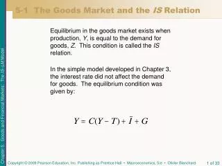
5-1 The Goods Market and the IS Relation. Equilibrium in the goods market exists when production, Y , is equal to the demand for goods, Z . This condition is called the IS relation.

E N D
5-1 The Goods Market and the IS Relation • Equilibrium in the goods market exists when production, Y, is equal to the demand for goods, Z. This condition is called the IS relation. • In the simple model developed in Chapter 3, the interest rate did not affect the demand for goods. The equilibrium condition was given by:
5-1 The Goods Market and the IS Relation Investment, Sales, and the Interest Rate Investment depends primarily on two factors: • The level of sales (+) • The interest rate (-)
5-1 The Goods Market and the IS Relation Determining Output Taking into account the investment relation, the equilibrium condition in the goods market becomes: For a given value of the interest rate i, demand is an increasing function of output, for two reasons: • An increase in output leads to an increase in income and also to an increase in disposable income. • An increase in output also leads to an increase in investment.
5-1 The Goods Market and the IS Relation Determining Output • Note two characteristics of ZZ: • Because it’s assumed that the consumption and investment relations in Equation (5.2) are linear, ZZ is, in general, a curve rather than a line. • ZZ is drawn flatter than a 45-degree line because it’s assumed that an increase in output leads to a less than one-for-one increase in demand.
5-1 The Goods Market and the IS Relation Figure 5 - 1 Equilibrium in the Goods Market Determining Output The demand for goods is an increasing function of output. Equilibrium requires that the demand for goods be equal to output.
5-1 The Goods Market and the IS Relation Determining Output • Note two characteristics of ZZ: • Because it’s assumed that the consumption and investment relations in Equation (5.2) are linear, ZZ is, in general, a curve rather than a line. • ZZ is drawn flatter than a 45-degree line because it’s assumed that an increase in output leads to a less than one-for-one increase in demand.
5-1 The Goods Market and the IS Relation Figure 5 - 2 The Derivation of the IS Curve Deriving the IS Curve An increase in the interest rate decreases the demand for goods at any level of output, leading to a decrease in the equilibrium level of output. Equilibrium in the goods market implies that an increase in the interest rate leads to a decrease in output. The IS curve is therefore downward sloping.
5-1 The Goods Market and the IS Relation Shifts of the IS Curve We have drawn the IS curve in Figure 5-2, taking as given the values of taxes, T, and government spending, G. Changes in either T or G will shift the IS curve. To summarize: • Equilibrium in the goods market implies that an increase in the interest rate leads to a decrease in output. This relation is represented by the downward-sloping IS curve. • Changes in factors that decrease the demand for goods, given the interest rate, shift the IS curve to the left. Changes in factors that increase the demand for goods, given the interest rate, shift the IS curve to the right.
5-1 The Goods Market and the IS Relation Figure 5 - 3 Shifts of the IS Curve Shifts of the IS Curve An increase in taxes shifts the IS curve to the left.
5-2 Financial Markets and the LM Relation • The interest rate is determined by the equality of the supply of and the demand for money: M = nominal money stock$YL(i) = demand for money$Y = nominal incomei = nominal interest rate
5-2 Financial Markets and the LM Relation Real Money, Real Income, and the Interest Rate • The equation gives a relation between money, nominal income, and the interest rate. The LM relation: In equilibrium, the real money supply is equal to the real money demand, which depends on real income, Y, and the interest rate, i: From chapter 2, recall that Nominal GDP = Real GDP multiplied by the GDP deflator: Equivalently:
5-2 Financial Markets and the LM Relation Figure 5 - 4 The Derivation of theLM Curve Deriving the LM Curve An increase in income leads, at a given interest rate, to an increase in the demand for money. Given the money supply, this increase in the demand for money leads to an increase in the equilibrium interest rate. Equilibrium in the financial markets implies that an increase in income leads to an increase in the interest rate. The LM curve is therefore upward sloping.
5-2 Financial Markets and the LM Relation Deriving the LM Curve Figure 5-4(b) plots the equilibrium interest rate, i, on the vertical axis against income on the horizontal axis. This relation between output and the interest rate is represented by the upward sloping curve in Figure 5-4(b). This curve is called the LMcurve.
5-2 Financial Markets and the LM Relation Figure 5 - 5 Shifts of the LM curve Shifts of the LM Curve An increase in money causes the LM curve to shift down.
5-2 Financial Markets and the LM Relation Shifts of the LM Curve ■Equilibrium in financial markets implies that, for a given real money supply, an increase in the level of income, which increases the demand for money, leads to an increase in the interest rate. This relation is represented by the upward- sloping LM curve. ■An increase in the money supply shifts the LM curve down; a decrease in the money supply shifts the LM curve up.
5-3 Putting the IS and the LM Relations Together Figure 5 - 6 The IS–LM Model Equilibrium in the goods market implies that an increase in the interest rate leads to a decrease in output. This is represented by the IS curve. Equilibrium in financial markets implies that an increase in output leads to an increase in the interest rate. This is represented by the LM curve. Only at point A, which is on both curves, are both goods and financial markets in equilibrium.
5-3 Putting the IS and the LM Relations Together Fiscal Policy, Activity, and the Interest Rate • Fiscal contraction, or fiscal consolidation, refers to fiscal policy that reduces the budget deficit. • An increase in the deficit is called a fiscal expansion. • Taxes affect the IS curve, not the LM curve.
5-3 Putting the IS and the LM Relations Together Figure 5 - 7 The IS–LM Model Fiscal Policy, Activity, and the Interest Rate Equilibrium in the goods market implies that an increase in the interest rate leads to a decrease in output. This is represented by the IS curve. Equilibrium in financial markets implies that an increase in output leads to an increase in the interest rate. This is represented by the LM curve. Only at point A, which is on both curves, are both goods and financial markets in equilibrium.
5-3 Putting the IS and the LM Relations Together Monetary Policy, Activity, and the Interest Rate • Monetary contraction, or monetary tightening, refers to a decrease in the money supply. • An increase in the money supply is called monetary expansion. • Monetary policy does not affect the IS curve, only the LM curve. For example, an increase in the money supply shifts the LM curve down.
5-3 Putting the IS and the LM Relations Together Figure 5 - 8 The Effects of a Monetary Expansion Monetary Policy, Activity, and the Interest Rate A monetary expansion leads to higher output and a lower interest rate.
Deficit Reduction: Good or Bad for Investment? Investment = Private saving + Public savingI = S + (T – G) A fiscal contraction may decrease investment. Or, looking at the reverse policy, a fiscal expansion—a decrease in taxes or an increase in spending—may actually increase investment.
5-4 Using a Policy Mix The combination of monetary and fiscal polices is known as the monetary-fiscal policy mix, or simply, the policy mix. Sometimes, the right mix is to use fiscal and monetary policy in the same direction. Sometimes, the right mix is to use the two policies in opposite directions—for example, combining a fiscal contraction with a monetary expansion.
The U.S. Recession of 2001 Figure 1 The U.S. Growth Rate, 1999:1 to 2002:4
The U.S. Recession of 2001 Figure 2 The Federal Funds Rate, 1999:1 to 2002:4
The U.S. Recession of 2001 Figure 3 U.S. Federal Government Revenues and Spending (as Ratios to GDP), 1999:1 to 2002:4
The U.S. Recession of 2001 Figure 4 The U.S. Recession of 2001
The U.S. Recession of 2001 • What happened in 2001 was the following: • The decrease in investment demand led to a sharp shift of the IS curve to the left, from IS to IS’. • The increase in the money supply led to a downward shift of the LM curve, from LM to LM’. • The decrease in tax rates and the increase in spending both led to a shift of the IS curve to the right, from IS’’ to IS’.
5-5 How Does the IS-LM Model Fit the Facts? Introducing dynamics formally would be difficult, but we can describe the basic mechanisms in words. • Consumers are likely to take some time to adjust their consumption following a change in disposable income. • Firms are likely to take some time to adjust investment spending following a change in their sales. • Firms are likely to take some time to adjust investment spending following a change in the interest rate. • Firms are likely to take some time to adjust production following a change in their sales.
5-5 How Does the IS-LM Model Fit the Facts? Figure 5 - 9 The Empirical Effects of an Increase in the Federal Funds Rate In the short run, an increase in the federal funds rate leads to a decrease in output and to an increase in unemployment, but it has little effect on the price level.
5-5 How Does the IS-LM Model Fit the Facts? The two dashed lines and the tinted space between the dashed lines represents a confidence band, a band within which the true value of the effect lies with 60% probability: • Figure 5-9(a) shows the effects of an increase in the federal funds rate of 1% on retail sales over time. The percentage change in retail sales is plotted on the vertical axis; time, measured in quarters, is on the horizontal axis. • Figure 5-9(b) shows how lower sales lead to lower output. • Figure 5-9(c) shows how lower output leads to lower employment: As firms cut production, they also cut employment. • The decline in employment is reflected in an increase in the unemployment rate, shown in Figure 5-9(d). • Figure 5-9(e) looks at the behavior of the price level.
Key Terms • IS curve • LM curve • fiscal contraction, fiscal consolidation • fiscal expansion • monetary expansion • monetary contraction, monetary tightening • monetary–fiscal policy mix, policy mix • confidence band