Download
1 / 66
670 likes | 962 Views
Turing Machines and Computability. Devices of Increasing Computational Power. So far: Finite Automata – good for devices with small amounts of memory, relatively simple control Pushdown Automata – stack-based automata

E N D
Devices of Increasing Computational Power • So far: • Finite Automata – good for devices with small amounts of memory, relatively simple control • Pushdown Automata – stack-based automata • But both have limitations for even simple tasks, too restrictive as general purpose computers • Enter the Turing Machine • More powerful than either of the above • Essentially a finite automaton but with unlimited memory • Although theoretical, can do everything a general purpose computer of today can do • If a TM can’t solve it, neither can a computer
Turing Machines • TM’s described in 1936 • Well before the days of modern computers but remains a popular model for what is possible to compute on today’s systems • Advances in computing still fall under the TM model, so even if they may run faster, they are still subject to the same limitations • A TM consists of a finite control (i.e. a finite state automaton) that is connected to an infinite tape.
Turing Machine • The tape consists of cells where each cell holds a symbol from the tape alphabet. Initially the input consists of a finite-length string of symbols and is placed on the tape. To the left of the input and to the right of the input, extending to infinity, are placed blanks. The tape head is initially positioned at the leftmost cell holding the input. Finite control … B B X1 X2 … Xi Xn B B …
Turing Machine Details • In one move the TM will: • Change state, which may be the same as the current state • Write a tape symbol in the current cell, which may be the same as the current symbol • Move the tape head left or right one cell • The special states for rejecting and accepting take effect immediately • Formally, the Turing Machine is denoted by the 8-tuple: • M = (Q, , Γ, δ, q0, B, qa, qr)
Turing Machine Description • Q = finite states of the control • = finite set of input symbols, which is a subset of Γ below • Γ = finite set of tape symbols • δ = transition function. δ(q,X) are a state and tape symbol X. • The output is the triple, (p, Y, D) • Where p = next state, Y = new symbol written on the tape, D = direction to move the tape head • q0= start state for finite control • B = blank symbol. This symbol is in Γ but not in . • qaccept = set of final or accepting states of Q. • qreject = set of rejecting states of Q
TM Example • Make a TM that recognizes the language L = { w#w | w (0,1)* }. That is, we have a language separated by a # symbol with the same string on both sides. • Here is a strategy we can employ to create the Turing machine: • Scan the input to make sure it contains a single # symbol. If not, reject. • Starting with the leftmost symbol, remember it and write an X into its cell. Move to the right, skipping over any 0’s or 1’s until we reach a #. Continue scanning to the first non-# symbol. If this symbol matches the original leftmost symbol, then write a # into the cell. Otherwise, reject. • Move the head back to the leftmost symbol that is not X. • If this symbol is not #, then repeat at step 2. Otherwise, scan to the right. If all symbols are # until we hit a blank, then accept. Otherwise, reject.
TM Example • Typically we will describe TM’s in this informal fashion. The formal description gets quite long and tedious. Nevertheless, we will give a formal description for this particular problem. • We can use a table format or a transition diagram format. In the transition diagram format, a transition is denoted by: Input symbol Symbol-To-Write Direction to Move For example: 0 1 R • Means take this transition if the input is 0, and replace the cell with a 1 and then move to the right. • Shorthand: 0 R means 0 0 R
TM for L={w#w:w0,1} 0R, 1R 0R, 1R 0L, 1L, #L Check for # a b c Start #R BL BR ## #R 0R, 1R 0R, 1R Match symbols Return to left No input left h d g f e 0X R 1X R #R #R 0L, 1L, #L 0# L 1# L i XR 1X R 0X R #R j k l #R BR
Instantaneous Description • Sometimes it is useful to describe what a TM does in terms of its ID (instantaneous description), just as we did with the PDA. • The ID shows all non-blank cells in the tape, pointer to the cell the head is over with the name of the current state • use the turnstile symbol ├ to denote the move. • As before, to denote zero or many moves, we can use ├*. • For example, for the above TM on the input 10#10 we can describe our processing as follows: Ba10#10B ├ B1a0#10B ├ B10a#10B ├ B10#b10B ├ B10#b10B ├ B10#1b0B ├ B10#10bB ├ B10#1c0B ├* cB10#10B ├ Bf10#10B ├* BXX#XXBl • In this example the blanks that border the input symbols are shown since they are used in the Turing machine to define the borders of our input.
Turing Machines and Halting • One way for a TM to accept input is to end in a final state. • Another way is acceptance by halting. We say that a TM halts if it enters a state q, scanning a tape symbol X, and there is no move in this situation; i.e. δ(q,X) is undefined. • Note that this definition of halting was not used in the transition diagram for the TM we described earlier; instead that TM died on unspecified input! • It is possible to modify the prior example so that there is no unspecified input except for our accepting state. An equivalent TM that halts exists for a TM that accepts input via final state. • In general, we assume that a TM always halts when it is in an accepting state. • Unfortunately, it is not always possible to require that a TM halts even if it does not accept the input. Turing machines that always halt, regardless of accepting or not accepting, are good models of algorithms for decidable problems. Such languages are called recursive.
Turing Machine Variants • There are many variations we can make to the basic TM • Extensions can make it useful to prove a theorem or perform some task • However, these extensions do not add anything extra the basic TM can’t already compute • Example: consider a variation to the Turing machine where we have the option of staying put instead of forcing the tape head to move left or right by one cell. • In the old model, we could replace each “stay put” move in the new machine with two transitions, one that moves right and one that moves left, to get the same behavior.
Multitape Turing Machines • A multitape Turing machine is like an ordinary TM but it has several tapes instead of one tape. • Initially the input starts on tape 1 and the other tapes are blank. • The transition function is changed to allow for reading, writing, and moving the heads on all the tapes simultaneously. • This means we could read on multiples tape and move in different directions on each tape as well as write a different symbol on each tape, all in one move.
Multitape Turing Machine • Theorem: A multitape TM is equivalent in power to an ordinary TM. Recall that two TM’s are equivalent if they recognize the same language. We can show how to convert a multitape TM, M, to a single tape TM, S: • Say that M has k tapes. • Create the TM S to simulate having k tapes by interleaving the information on each of the k tapes on its single tape • Use a new symbol # as a delimiter to separate the contents of each tape • S must also keep track of the location on each of the simulated heads • Write a type symbol with a * to mark the place where the head on the tape would be • The * symbols are new tape symbols that don’t exist with M • The finite control must have the proper logic to distinguish say, x* and x and realize both refer to the same thing, but one is the current tape symbol.
Multitape Machine Equivalent Single Tape Machine:
Single Tape Equivalent • One final detail • If at any point S moves one of the virtual tape heads onto a #, then this action signifies that M has moved the corresponding head onto the previously unread blank portion of that tape. • To accommodate this situation, S writes a blank symbol on this tape cell and shifts the tape contents to the rightmost # by one, adds a new #, and then continues back where it left off
Nondeterministic TM • Replace the “DFA” part of the TM with an “NFA” • Each time we make a nondeterministic move, you can think of this as a branch or “fork” to two simultaneously running machines. Each machine gets a copy of the entire tape. If any one of these machines ends up in an accepting state, then the input is accepted. • Although powerful, nondeterminism does not affect the power of the TM model • Theorem: Every nondeterministic TM has an equivalent deterministic TM. • We can prove this theorem by simulating any nondeterministic TM, N, with a deterministic TM, D.
Nondeterministic TM • Visualize N as a tree with branches whenever we fork off to two (or more) simultaneous machines. • Use D to try all possible branches of N, sequentially. • If D ever finds the accept state on one of these branches, then D accepts. • It is quite likely that D will never terminate in the event of a loop if there is no accepting state. • Search be done in a breadth-first rather than depth-first manner. • An individual branch may extend to infinity, and if we start down this branch then D will be stuck forever when some other branch may accept the input. • We can simulate N on D by a tape with a queue of ID’s and a scratch tape for temporary storage. • Each ID contains all the moves we have made from one state to the next, for one “branch” of the nondeterministic tree. • From the previous theorem, we can make as many multiple tapes as we like and this is still equivalent to a single tape machine. Initially, D looks like the following:
Nondeterministic TM • ID1 is the sequence of moves we make from the start state. The * indicates that this is the current ID we are executing. • We make a move on the TM. If this move results in a “fork” by following nondeterministic paths, then we create a new ID and copy it to the end of the queue using the scratch tape. D Scratch Tape … ID1* Queue of ID’s
Nondeterministic TM • For example, say that in ID1 we have two nondeterministic moves, resulting in ID2 and ID3: D Scratch Tape … ID1* # ID2 # ID3
Nondeterministic TM • After we’re done with a single move in ID1, which may result in increasing the length of ID1 and storing it back to the tape, we move on to ID2: D Scratch Tape … ID1 # ID2* # ID3
Nondeterministic TM • If any one of these states is accepting in an ID, then the machine quits and accepts. • If we ever reach the last ID, then we repeat back with the first ID. • Note that although the constructed deterministic TM is equivalent to accepting the same language as a nondeterministic TM, the deterministic TM might take exponentially more time than the nondeterministic TM. • It is unknown if this exponential slowdown is necessary. We’ll come back to this in the discussion of P vs. NP. • Theorem: Since any deterministic Turing Machine is also nondeterministic (there just happens to be no nondeterministic moves), there exists a nondeterministic TM for every deterministic TM.
Equivalence of TM’s and Computers • In one sense, a real computer has a finite amount of memory, and thus is weaker than a TM. • But, we can postulate an infinite supply of tapes, disks, or some peripheral storage device to simulate an infinite TM tape. Additionally, we can assume there is a human operator to mount disks, keep them stacked neatly on the sides of the computer, etc. • Need to show both directions, a TM can simulate a computer and that a computer can simulate a TM
Computer Simulate a TM • This direction is fairly easy - Given a computer with a modern programming language, certainly, we can write a computer program that emulates the finite control of the TM. • The only issue remains the infinite tape. Our program must map cells in the tape to storage locations in a disk. When the disk becomes full, we must be able to map to a different disk in the stack of disks mounted by the human operator.
TM Simulate a Computer • In this exercise the simulation is performed at the level of stored instructions and accessing words of main memory. • TM has one tape that holds all the used memory locations and their contents. • Other TM tapes hold the instruction counter, memory address, computer input file, and scratch data. • The computer’s instruction cycle is simulated by: • Find the word indicated by the instruction counter on the memory tape. • Examine the instruction code (a finite set of options), and get the contents of any memory words mentioned in the instruction, using the scratch tape. • Perform the instruction, changing any words' values as needed, and adding new address-value pairs to the memory tape, if needed.
TM/Computer Equivalence • Anything a computer can do, a TM can do, and vice versa • TM is much slower than the computer, though • But the difference in speed is polynomial • Each step done on the computer can be completed in O(n2) steps on the TM (see book for details of proof). • While slow, this is key information if we wish to make an analogy to modern computers. Anything that we can prove using Turing machines translates to modern computers with a polynomial time transformation. • Whenever we talk about defining algorithms to solve problems, we can equivalently talk about how to construct a TM to solve the problem. If a TM cannot be built to solve a particular problem, then it means our modern computer cannot solve the problem either.
Computability • Slight change in direction for the course • We will start to examine problems that are at the threshold and beyond the theoretical limits of what is possible to compute using computers today. • We will examine the following issues with the help of TM’s
Turing Languages • We use the simplicity of the TM model to prove formally that there are specific problems (i.e. languages) that the TM cannot solve. Three classes of languages: • Turing-decidable or recursive: TM can accept the strings in the language and tell if a string is not in the language. Sometimes these are called decidable problems. • Turing-recognizable or recursively enumerable : TM can accept the strings in the language but cannot tell for certain that a string is not in the language. Sometimes these are called partially-decidable. • Undecidable : no TM can even recognize ALL members of the language.
P and NP • We then look at problems (languages) that do have TM's that accept them and always halt; • i.e. they not only recognize the strings in the language, but they tell us when they are sure the string is not in the language. • The classes P and NP are those languages recognizable by deterministic and nondeterministic TM's, respectively, that halt within a time that is some polynomial in the input. • Polynomial is as close as we can get, because real computers and different models of (deterministic) TM's can differ in their running time by a polynomial function, e.g., a problem might take O(n2) time on a real computer and O(n6) time on a TM.
NP Complete • These are in a sense the “hardest” problems in NP. • These problems correspond to languages that are recognizable by a nondeterministic TM. • However, we will also be able to show that in polynomial time we can reduce any NP-complete problem to any other problem in NP. • This means that if we could prove an NP Complete problem to be solvable in polynomial time, then P = NP. • We will examine some specific problems that are NP-complete: satisfiability of boolean (propositional logic) formulas, traveling salesman, etc.
Hilbert’s Problems • In 1900, mathematician David Hilbert identified 23 mathematical challenges • Problem 10: Devise an algorithm to determine if a given diophantine polynomial has integral roots • We know now that no algorithm exists for this task! It is algorithmically unsolvable. • 1970 by Yuri Matijasevic • Tools didn’t exist in 1900 to adequately describe an algorithm to prove that no such algorithm exists • Church’s Lambda Calculus and Turing’s Turing machines formalized computation and have been shown to be equivalent • The Church-Turing Thesis Intuitive Notion of Algorithms = Turing Machine Algorithms
Hilbert’s Problem as a TM • D = { p | p is a polynomial with an integral root } • Determine whether the set D is decidable • (Can’t do it) • We can show that D is Turing-recognizable • Consider Hilbert’s problem only for variable X • D1 = {p| p is a polynomial over x with integral roots} • TM(D1) : Evaluate p with x set successively to the values 0, 1, -1, 2, -3, 3, -3, … if at any point the polynomial evaluates to 0, accept • If D1 has an integral root, this TM will eventually find it • If D1 has no integral root, this TM will run forever • This TM is a recognizer not a decider • We can convert it to a decider if we set bounds, but Matijasevic showed calculating such bounds for multivariable polynomials is impossible
Decidable Languages • Review: What is a decidable language? • Theorems: • ADFA = {<B,w> | B is a DFA that accepts input string w } • This is the language that corresponds to any DFA we could build • We can make a TM that simulates DFA B on w and indicates if we should accept or reject • ANFA can be proven similarly • AREX can be proven similarly < > Indicates description of DFA
Decidable Problems • ACFG= {<G,w> | G is a CFG that generates w} • This is decidable • Can’t go through all derivations to see if one of them is w, since there may be an infinite number of derivations • But we can convert G to Chomsky Normal Form, any derivation for w has at most 2|w| – 1 steps, so we can generate all derivations using 2|w| - 1 steps and see if one of these matches w • We can also show that every CFG is decidable • See text
Relationship among classes of Languages Decidable Context-Free Regular Turing Recognizable Let’s look at some undecidable languages…
Intuitive Argument for an Undecidable Problem • Given a C program (or a program in any programming language, really) that prints “hello, world” is there another program that can test if a program given as input prints “hello, world”? • This is tougher than it may sound at first glance. For some programs it is easy to determine if it prints hello world. Here is perhaps the simplest: #include “stdio.h” void main() { printf(“hello, world\n”); }
Not as easy as it looks… • It would be fairly easy to write a program to test to see if another program consisting solely of printf statements will output “hello, world”. But what we want is a program that can take any arbitrary program and determine if it prints “hello, world”. • This is much more difficult. Consider the following program:
Obfuscated Hello World Program #include "stdio.h" #define e 3 #define g (e/e) #define h ((g+e)/2) #define f (e-g-h) #define j (e*e-g) #define k (j-h) #define l(x) tab2[x]/h #define m(n,a) ((n&(a))==(a)) long tab1[]={ 989L,5L,26L,0L,88319L,123L,0L,9367L }; int tab2[]={ 4,6,10,14,22,26,34,38,46,58,62,74,82,86 }; main(m1,s) char *s; { int a,b,c,d,o[k],n=(int)s; if(m1==1){ char b[2*j+f-g]; main(l(h+e)+h+e,b); printf(b); } else switch(m1-=h){ case f: a=(b=(c=(d=g)<<g)<<g)<<g; return(m(n,a|c)|m(n,b)|m(n,a|d)|m(n,c|d)); case h: for(a=f;a<j;++a)if(tab1[a]&&!(tab1[a]%((long)l(n))))return(a); case g: if(n<h)return(g); if(n<j){n-=g;c='D';o[f]=h;o[g]=f;} else{c='\r'-'\b';n-=j-g;o[f]=o[g]=g;} if((b=n)>=e)for(b=g<<g;b<n;++b)o[b]=o[b-h]+o[b-g]+c; return(o[b-g]%n+k-h); default: if(m1-=e) main(m1-g+e+h,s+g); else *(s+g)=f; for(*s=a=f;a<e;) *s=(*s<<e)|main(h+a++,(char *)m1); } }
Aside • From Wikipedia, the International Obfuscated C Code Contest • Some quotes from 2004 winners include: • To keep things simple, I have avoided the C preprocessor and tricky statements such as "if", "for", "do", "while", "switch", and "goto". • Why not use the program to hide another program in the program? It must have seemed reasonable at the time. • The program implements an 11-bit ALU in the C preprocessor. • I found that calculating prime numbers up to 1024 makes the program include itself over 6.8 million times.
Hello World Tester • Problem: Create a program that determines if any arbitrary program prints “hello world” • We can show there is no program to solve that problem (i.e. it is undecidable) • Suppose that there were such a program H, the “hello-world-tester." • H takes as input a program P and an input file I for that program, and tells whether P, with input I, prints “hello world” and outputs “yes” if it does, “no” if it does not
Hello World Tester I yes H Hello-world tester no P
Hello World Tester • Next we modify H to a new program H1 that acts like H, but when H prints no, H1 prints “hello, world.”. • To do this, we need to find where “no” is printed and instead output “hello world” instead: I yes H1 Hello-world tester hello, world P
Hello World Tester • Next modify H1 to H2 . The program H2 takes only one input, P2, instead of both P and I. • To do this, the new input P2 must include the data input I and the program P. • The program P and data input I are all stored in a buffer in program H2. H2 then simulates H1, but whenever H1 reads input, H2 feeds the input from the buffered copy. H2 can maintain two index pointers into the buffered data to know what current data and code should be read next: H2 H1 yes P2=P,I Buffer: P I hello, world
Hello World Tester • However, H2 cannot exist. If it did, what would H2(H2 ) do? • That is, we give H2 as input to itself: yes H2 Hello-world tester H2 hello, world If H2 on the left outputs = “yes”, then H2 given H2 as input will print “hello, world”. But we just supposed that the first output H2 makes is “yes” and not “hello world”. The situation is paradoxical and we conclude that H2 cannot exist and this problem is undecidable.
Software Verification • You are given a computer program and a precise specification of what the program is supposed to do. You need to verify that the program performs correctly to the specification. • But the general problem of software verification is not solvable by computer. • This is a general case of the Halting Problem
The Halting Problem • ATM = {<M, w> | M is a TM and M accepts w } • i.e. Can we make a TM that can determine if another TM will accept a string w? • The problem is the TM might get stuck in a loop and go forever; we could simulate the original TM, but if it loops, we are stuck • However, this problem is Turing Recognizable: • Simulate M on input w. • If M ever enters its accept state, accept. If M ever enters its reject state, reject. • M might loop; if it had some way to determine that M was not halting on w, it could reject. To show that the Halting Problem is unsolvable, first, counting…
Countability • Countability described by Georg Cantor in 1873. • If we have two infinite sets, how can we tell whether one is larger than the other? (e.g. floats larger than ints) • Obviously we can’t start counting with each element or we will be counting forever. • Cantor’s solution is to make a correspondence to the set of natural numbers. • A correspondence is a function f: AB that is one-to-one from A to B. Every element of A maps to a unique element of B, and each element of B has a unique element of A mapping to it.
Countability Example • The set of natural numbers, N = { 1, 2, 3, 4, … }. • The set of even numbers excluding 0, E = { 2, 4, 6, … } • It might seem that N is bigger than E, since we have values in N that are not in E (by one measure, we have twice as many.) However, using Cantor’s definition of size both sets have the same size.
Countability • Definition: A set is countable if it is finite or if it has the same size as the natural numbers. • For example, as we saw above, E is countable. • For every number in N, there is a corresponding number in E
Countability • Example: The set of positive rational numbers, Q, is countable. That is, Q = { m/n | m, n N }. • To show that this is countable, we need to make a 1:1 correspondence between the rational numbers and the natural numbers. We must make sure that each rational number is paired with one and only one natural number. • Consider the mapping as shown in the following matrix: