Download

1 / 11
120 likes | 293 Views
Graph Algebra III: Nonlinearities. Courtney Brown, Ph.D. Emory University. Nonlinearities with Systems Begin with the Inputs. Whenever there is an input, there is the potential for nonlinearities.

E N D
Graph Algebra III: Nonlinearities Courtney Brown, Ph.D. Emory University
Nonlinearities with Systems Begin with the Inputs • Whenever there is an input, there is the potential for nonlinearities. • The inputs drive the system. The boundary of the system may be linear, but the inputs can be anything. • In such situations, an input function or actual data can drive the overtime behavior of the system to appear nonlinear, even though the system itself is processing the input linearly.
A Linear System and a Time-Dependent Input • The input can vary nonlinearly. • Remember that linear systems can behave nonlinearly over time. Nonlinear inputs compound this effect.
A Nonlinear System Using a Time-Dependent Parameter • This system uses a variable operator of the proportional transformation. This is a parameter that changes with time (i.e., is not constant).
Interpreting the Nonlinear System • Using Mason’s Rule, this system can be written as Outputt = [p/(1-pm)]StInputt • Here, the input could be tensions in a society. • St could be the effect of socialization in absorbing those tensions • Outputt could be social conflict.
Using a Function to Model a Parameter • You could use a function to describe change in St. • For example, St = S0 + S1t+1 • If S1 is a number between 0 and 1, we would have a function for St that would be decreasing in time, drawn to the equilibrium value of S0. • Stallows the input to pass into the system.
Alternative Approaches Always Exist • One could also model the parameter St as first-order linear difference equation with constant coefficients. • Thus, we could say St+1 = aSt + b. • Here the equilibrium would be S* = b/(1-a).
Nonlinear States • Nonlinearities can also be introduced into a model using nonlinear states. • Here, the output is also on the forward path.
Let us say that Ut = potential total recruits or supporters • Yt = the already mobilized • X1 = Ut – Yt = the proportion of the population who are available for mobilization but not yet mobilized • X2 = X1pYt = (Ut – Yt)Ytp which is the probability that an interaction between a mobilized person (e.g. a voter) and a nonmobilized person (e.g. a nonvoter) will result in a newly mobilized person (e.g., a convert of a voter) • X3 = the sum of the converted
The equation for this model is Yt = [Δ-1pYt/(1+ Δ-1pYt)]Ut which yields Yt+1 = Yt(1+pUt) – pYt2. • This is a quadratic. • Estimation would be easier if it is written as Yt+1 = Yt + pYtUt – pYt2. • In SAS, you would use a restrict statement in Proc Reg to make the slope for Ytequal to 1. You would also have to force the estimated slope for YtUt to have the same value but opposite sign of Yt2. These are a requirements of the formal model.