Download
1 / 27
270 likes | 434 Views
Design and Analysis of Clinical Study 5. Introduction to R and Statistics. Dr. Tuan V. Nguyen Garvan Institute of Medical Research Sydney, Australia. Introduction: Historical development S, Splus Capability Statistical Analysis References Calculator Data Type Resources

E N D
Design and Analysis of Clinical Study 5. Introduction to R and Statistics Dr. Tuan V. Nguyen Garvan Institute of Medical Research Sydney, Australia
Introduction: Historical development S, Splus Capability Statistical Analysis References Calculator Data Type Resources Simulation and Statistical Tables Probability distributions Outline
S: an interactive environment for data analysis developed at Bell Laboratories since 1976 1988 - S2: RA Becker, JM Chambers, A Wilks 1992 - S3: JM Chambers, TJ Hastie 1998 - S4: JM Chambers Exclusively licensed by AT&T/Lucent to Insightful Corporation, Seattle WA. Product name: "S-plus". R: initially written by Ross Ihaka and Robert Gentleman at Dep. of Statistics of U of Auckland, New Zealand during 1990s. Since 1997: international "R-core" team of ca. 15 people with access to common CVS archive. History
Introduction • R is "GNU S" — A language and environment for data manipula-tion, calculation and graphical display. • a suite of operators for calculations on arrays & matrices. • a large, coherent, integrated collection of data analysis tools • graphical facilities for data analysis • a well developed programming language
What R does and does not • is not a database, but connects to DBMSs • has no graphical user interfaces, but connects to Java, TclTk • language interpreter can be very slow, but allows to call own C/C++ code • no spreadsheet view of data, but connects to Excel/MsOffice • no professional / commercial support • data handling and storage: numeric, textual • matrix algebra • hash tables and regular expressions • high-level data analytic and statistical functions • graphics • programming language: loops, branching, subroutines
R and Statistics • Packaging: a crucial infrastructure to efficiently produce, load and keep consistent software libraries from (many) different sources / authors • Statistics: most packages deal with statistics and data analysis • State of the art: many statistical researchers provide their methods as R packages
Data Analysis and Presentation • The R distribution contains functionality for large number of statistical procedures. • linear and generalized linear models • nonlinear regression models • time series analysis • classical parametric and nonparametric tests • clustering • smoothing • R also has a large set of functions which provide a flexible graphical environment for creating various kinds of data presentations.
R as a calculator > log2(32) [1] 5 > sqrt(2) [1] 1.414214 > seq(0, 5, length=6) [1] 0 1 2 3 4 5 > plot(sin(seq(0, 2*pi, length=100)))
Objects Primitive (or: atomic) data types in R are: • numeric (integer, double, complex) • character • logical • function out of these, vectors, arrays, lists can be built.
R "grammar" object <- function(argument1, argument2, ..., argumentn) Example: > reg <- lm(y ~ x) x == 5 x bằng 5 x != 5 x không bằng 5 y < x y nhỏ hơn x x > y x lớn hơn y z <= 7 z nhỏ hơn hoặc bằng 7 p >= 1 p lớn hơn hoặc bằng 1 is.na(x) Có phải x là biến số missing A & B A và B (AND) A | B A hoặc B (OR) ! Không là (NOT)
Reading Data 1 – Direct Method age insulin 50 16.5 62 10.8 60 32.3 40 19.3 48 14.2 47 11.3 57 15.5 70 15.8 48 16.2 67 11.2 > age <- c(50,62, 60,40,48,47,57,70,48,67) > insulin <-c(16.5,10.8,32.3,19.3,14.2,11.3,15.5,15.8,16.2,11.2) > ins <- data.frame(age, insulin)
Reading Data 2 – read.table id sex age bmi hdl ldl tc tg 1 Nam 57 17 5.000 2.0 4.0 1.1 2 Nu 64 18 4.380 3.0 3.5 2.1 3 Nu 60 18 3.360 3.0 4.7 0.8 4 Nam 65 18 5.920 4.0 7.7 1.1 5 Nam 47 18 6.250 2.1 . 2.1 6 Nu 65 18 4.150 3.0 4.2 1.5 7 Nam 76 19 0.737 3.0 5.9 2.6 > setwd("c:/works/stats") > chol <- read.table("chol.txt", header=TRUE, na.missing=".")
Reading Data 3 – read.csv • Bước 1: Dùng lệnh "Save as" trong Excel và lưu số liệu dưới dạng "csv"; • Bước 2: Dùng R (lệnh read.csv) để nhập dữ liệu dạng csv > setwd("c:/works/stats") > gh <- read.csv ("excel.csv", header=TRUE)
A Simple Session sex <- c("Nam", "Nu", "Nu","Nam","Nam", "Nu","Nam","Nam","Nam", "Nu", "Nu","Nam", "Nu","Nam","Nam", "Nu", "Nu", "Nu", "Nu", "Nu", "Nu", "Nu", "Nu", "Nu","Nam","Nam", "Nu","Nam", "Nu", "Nu", "Nu","Nam","Nam", "Nu", "Nu","Nam", "Nu","Nam", "Nu", "Nu", "Nam", "Nu","Nam","Nam","Nam", "Nu","Nam","Nam", "Nu", "Nu") age <- c(57, 64, 60, 65, 47, 65, 76, 61, 59, 57, 63, 51, 60, 42, 64, 49, 44, 45, 80, 48, 61, 45, 70, 51, 63, 54, 57, 70, 47, 60, 60, 50, 60, 55, 74, 48, 46, 49, 69, 72, 51, 58, 60, 45, 63, 52, 64, 45, 64, 62) bmi <- c( 17, 18, 18, 18, 18, 18, 19, 19, 19, 19, 20, 20, 20, 20, 20, 20, 21, 21, 21, 21, 21, 21, 21, 21, 22, 22, 22, 22, 22, 22, 22, 22, 22, 22, 23, 23, 23, 23, 23, 23, 23, 23, 24, 24, 24, 24, 24, 24, 25, 25) hdl <- c(5.000, 4.380, 3.360, 5.920, 6.250, 4.150, 0.737, 7.170, 6.942, 5.000, 4.217, 4.823, 3.750, 1.904, 6.900, 0.633, 5.530, 6.625, 5.960, 3.800, 5.375, 3.360, 5.000, 2.608, 4.130,5.000, 6.235, 3.600, 5.625, 5.360, 6.580, 7.545, 6.440,6.170,5.270, 3.220, 5.400, 6.300, 9.110, 7.750, 6.200, 7.050, 6.300, 5.450,5.000,3.360,7.170,7.880,7.360,7.750) ldl <- c(2.0, 3.0, 3.0, 4.0, 2.1, 3.0, 3.0, 3.0, 3.0, 2.0, 5.0, 1.3, 1.2, 0.7, 4.0, 4.1, 4.3, 4.0, 4.3, 4.0, 3.1, 3.0, 1.7, 2.0, 2.1, 4.0, 4.1, 4.0, 4.2, 4.2, 4.4, 4.3, 2.3, 6.0, 3.0, 3.0, 2.6, 4.4, 4.3, 4.0, 3.0, 4.1, 4.4, 2.8, 3.0, 2.0, 1.0, 4.0, 4.6, 4.0) tc <-c (4.0, 3.5, 4.7, 7.7, 5.0, 4.2, 5.9, 6.1, 5.9, 4.0, 6.2, 4.1, 3.0, 4.0, 6.9, 5.7, 5.7, 5.3, 7.1, 3.8, 4.3, 4.8, 4.0, 3.0, 3.1, 5.3, 5.3, 5.4, 4.5, 5.9, 5.6, 8.3, 5.8, 7.6, 5.8, 3.1, 5.4, 6.3, 8.2, 6.2, 6.2, 6.7, 6.3, 6.0, 4.0, 3.7, 6.1, 6.7, 8.1, 6.2) tg <- c(1.1, 2.1, 0.8, 1.1, 2.1, 1.5, 2.6, 1.5, 5.4, 1.9, 1.7, 1.0, 1.6, 1.1, 1.5, 1.0, 2.7, 3.9, 3.0, 3.1, 2.2, 2.7, 1.1, 0.7, 1.0, 1.7, 2.9, 2.5, 6.2, 1.3, 3.3, 3.0, 1.0, 1.4, 2.5, 0.7, 2.4, 2.4, 1.4, 2.7, 2.4, 3.3, 2.0, 2.6, 1.8, 1.2, 1.9, 3.3, 4.0, 2.5) cong <- data.frame(sex, age, bmi, hdl, ldl, tc, tg) attach(cong)
Bar Graph > sex.freq <- table(sex) > sex.freq sex Nam Nu 22 28 > barplot(sex.freq, main="Frequency of males and females") > barplot(table(sex), main="Frequency of males and females") > stripchart(tg, main="Strip chart for triglycerides", xlab="mg/L")
Histogram, Boxplot > hist(age) > hist(age, main="Frequency distribution by age group", xlab="Age group", ylab="No of patients") > plot(density(age),add=TRUE) > boxplot(tc, main="Box plot of total cholesterol", ylab="mg/L") > boxplot(tc~sex, horizontal=TRUE, main="Box plot of total cholesterol", ylab="mg/L", col = "pink")
Multiple Graphs > op <- par(mfrow=c(2,3)) > hist(tc) > hist(hdl) > hist(ldl) > hist(tg) > hist(bmi) > hist(age)
Scatter Plots > plot(tc, hdl) > plot(hdl, tc, pch=ifelse(sex=="Nam", 16, 22)) > plot(hdl, tc, pch=ifelse(sex=="Nam", "M", "F")) > plot(hdl ~ tc, pch=16, main="Total cholesterol and HDL cholesterol with LOEWSS smooth function", xlab="Total cholesterol", ylab="HDL cholesterol", bty="l") > lines(lowess(hdl, tc, f=2/3, iter=3), col="red") > lipid <- data.frame(age,bmi,hdl,ldl,tc) > pairs(lipid, pch=16)
Descriptive Statistics > mean(tc) [1] 5.414 > var(tc) [1] 1.962045 > sd(tc) [1] 1.40073 > summary(cong) sex age bmi hdl ldl Nam:22 Min. :42.00 Min. :17.00 Min. :0.633 Min. :0.700 Nu :28 1st Qu.:49.25 1st Qu.:20.00 1st Qu.:4.167 1st Qu.:2.650 Median :59.50 Median :22.00 Median :5.425 Median :3.050 Mean :57.64 Mean :21.38 Mean :5.333 Mean :3.292 3rd Qu.:63.75 3rd Qu.:23.00 3rd Qu.:6.545 3rd Qu.:4.100 Max. :80.00 Max. :25.00 Max. :9.110 Max. :6.000 tc tg Min. :3.000 Min. :0.700 1st Qu.:4.125 1st Qu.:1.325 Median :5.650 Median :2.050 Mean :5.414 Mean :2.176 3rd Qu.:6.200 3rd Qu.:2.700 Max. :8.300 Max. :6.200
Descriptive Statistics by Group, t-test > tapply(tc, list(sex), mean) Nam Nu 5.554545 5.303571 > t.test(tc ~ sex, data=cong) Welch Two Sample t-test data: tc by sex t = 0.6283, df = 46.09, p-value = 0.5329 alternative hypothesis: true difference in means is not equal to 0 95 percent confidence interval: -0.553024 1.054972 sample estimates: mean in group Nam mean in group Nu 5.554545 5.303571
Wilcoxon test > wilcox.test(tc ~ sex, data=cong) Wilcoxon rank sum test with continuity correction data: tc by sex W = 355, p-value = 0.3629 alternative hypothesis: true mu is not equal to 0 Warning message: cannot compute exact p-value with ties in: wilcox.test.default(x = c(4, 7.7, 5, 5.9, 6.1, 5.9, 4.1, 4, 6.9,
Test for Two Proportions > fracture <- c(7, 20) > total <- c(100, 110) > prop.test(fracture, total) 2-sample test for equality of proportions with continuity correction data: fracture out of total X-squared = 4.8901, df = 1, p-value = 0.02701 alternative hypothesis: two.sided 95 percent confidence interval: -0.20908963 -0.01454673 sample estimates: prop 1 prop 2 0.0700000 0.1818182
Comparison of Multiple Proportions > female <- c( 4, 43, 22, 0) > total <- c(8, 60, 30, 2) > prop.test(female, total) 4-sample test for equality of proportions without continuity correction data: female out of total X-squared = 6.2646, df = 3, p-value = 0.09942 alternative hypothesis: two.sided sample estimates: prop 1 prop 2 prop 3 prop 4 0.5000000 0.7166667 0.7333333 0.0000000 Warning message: Chi-squared approximation may be incorrect in: prop.test(female, total)
Linear Regression Analysis > age <- c(46,20,52,30,57,25,28,36,22,43,57,33,22,63,40,48,28,49) > bmi <-c(25.4,20.6,26.2,22.6,25.4,23.1,22.7,24.9,19.8,25.3,23.2, 21.8,20.9,26.7,26.4,21.2,21.2,22.8) > chol <- c(3.5,1.9,4.0,2.6,4.5,3.0,2.9,3.8,2.1,3.8,4.1,3.0, 2.5,4.6,3.2, 4.2,2.3,4.0) > data <- data.frame(age, bmi, chol) > plot(chol ~ age, pch=16)
Coefficient of Correlation > cor.test(age, chol) Pearson's product-moment correlation data: age and chol t = 10.7035, df = 16, p-value = 1.058e-08 alternative hypothesis: true correlation is not equal to 0 95 percent confidence interval: 0.8350463 0.9765306 sample estimates: cor 0.936726
Simple Linear Regression Analysis > reg <- lm(chol ~ age) > summary(reg) Call: lm(formula = chol ~ age) Residuals: Min 1Q Median 3Q Max -0.40729 -0.24133 -0.04522 0.17939 0.63040 Coefficients: Estimate Std. Error t value Pr(>|t|) (Intercept) 1.089218 0.221466 4.918 0.000154 *** age 0.057788 0.005399 10.704 1.06e-08 *** --- Signif. codes: 0 '***' 0.001 '**' 0.01 '*' 0.05 '.' 0.1 ' ' 1 Residual standard error: 0.3027 on 16 degrees of freedom Multiple R-Squared: 0.8775, Adjusted R-squared: 0.8698 F-statistic: 114.6 on 1 and 16 DF, p-value: 1.058e-08
Multiple Linear Regression Analysis > mreg <- lm(chol ~ age + bmi) > summary(mreg) Call: lm(formula = chol ~ age + bmi) Residuals: Min 1Q Median 3Q Max -0.3762 -0.2259 -0.0534 0.1698 0.5679 Coefficients: Estimate Std. Error t value Pr(>|t|) (Intercept) 0.455458 0.918230 0.496 0.627 age 0.054052 0.007591 7.120 3.50e-06 *** bmi 0.033364 0.046866 0.712 0.487 --- Signif. codes: 0 '***' 0.001 '**' 0.01 '*' 0.05 '.' 0.1 ' ' 1 Residual standard error: 0.3074 on 15 degrees of freedom Multiple R-Squared: 0.8815, Adjusted R-squared: 0.8657 F-statistic: 55.77 on 2 and 15 DF, p-value: 1.132e-07