Download
1 / 62
650 likes | 926 Views
Business Statistics: A Decision-Making Approach 8 th Edition. Chapter 9 Introduction to Hypothesis Testing. Chapter Goals. After completing this chapter, you should be able to: Formulate null and alternative hypotheses involving a single population mean or proportion

E N D
Business Statistics: A Decision-Making Approach 8th Edition Chapter 9Introduction to Hypothesis Testing
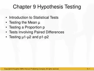
Chapter Goals After completing this chapter, you should be able to: • Formulate null and alternative hypotheses involving a single population mean or proportion • Know what Type I and Type II errors are • Formulate a decision rule for testing a hypothesis • Know how to use the test statistic, critical value, and p-value approaches to test the null hypothesis • Compute the probability of a Type II error
What is Hypothesis Testing? • A statistical hypothesis is an assumption about a population parameter (assumption may or may not be true). • The best way to determine whether a statistical hypothesis is true would be to examine the entire population. • Often impractical. So, examine a random sample • If sample data are not consistent with the statistical hypothesis, the hypothesis is rejected. • We never 100% “prove” anything because of sampling error
Types of Hypotheses • Null hypothesis. • Denoted by H0 • Alternative hypothesis. • Denoted by H1 or Ha
The Null Hypothesis, H0 • States the assumption to be tested • Example: The average number of TV sets in U.S. Homes is at least three ( ) • Is always about a population parameter, not about a sample statistic (even though sample is used)
The Null Hypothesis, H0 (continued) • Begin with the assumption that the null hypothesis is true • Similar to the notion of “innocent until proven guilty” • Always contains “=” , “≤” or “”sign • May or may not be rejected • Based on the statistical evidence gathered
The Alternative Hypothesis, HA • Is the opposite of the null hypothesis • e.g.: The average number of TV sets in U.S. homes is less than 3 ( HA: µ < 3 ) • Contains “≠”, “<” or “>” sign • Never contains the “=” , “≤” or “” sign • May or may not be accepted
Formulating Hypotheses • Example 1: The average annual income of buyers of Ford F150 pickup trucks is claimed to be $65,000 per year. An industry analyst would like to test this claim. • What is the appropriate test? • H0: µ = 65,000 (income is as claimed) • HA: µ ≠ 65,000 (income is different than claimed) • The analyst will believe the claim unless sufficient evidence is found to discredit it.
Formulating Hypotheses • Example 2: Ford Motor Company has worked to reduce road noise inside the cab of the redesigned F150 pickup truck. It would like to report in its advertising that the truck is quieter. The average of the prior design was 68 decibels at 60 mph. • What is the appropriate test? • H0: µ ≤ 67 (the truck is quieter: must be less than 68) • HA: µ > 68 (the truck is not quieter)
Steps for Formulating Hypothesis Tests • State the hypotheses. • The hypotheses must be mutually exclusive. • That is, if one is true, the other must be false. • Formulate an analysis plan. • The analysis plan describes how to use sample data to evaluate the null hypothesis. • The evaluation often focuses around a single test statistic.
Steps for Formulating Hypothesis Tests • Analyze sample data. • Find the value of the test statistic (mean score, proportion, t-score, z-score, etc.) described in the analysis plan and interpret result. • Apply the decision rule described in the analysis plan. • If the value of the test statistic is unlikely, based on the null hypothesis, reject the null hypothesis.
Errors in Making Decisions • 3 outcomes for a hypothesis test • No error (no need to discuss) • Type I error (Khan academy: type I error) • Type II error
Errors in Making Decisions (continued) • Type I Error • Rejecting a true null hypothesis • Considered as a serious error The probability of Type I Error is • Called level of significance of the test • Set by researcher in advance
Errors in Making Decisions (continued) • Type II Error • Failing to reject (i.e., accept) a false null hypothesis The probability of Type II Error is β • βis a calculated value, the formula is discussed later in the chapter
Outcomes and Probabilities Possible Hypothesis Test Outcomes State of Nature Decision H0 True H0 False Do Not No error (1 - ) Type II Error ( β ) Reject Key: Outcome (Probability) a H 0 Reject Type I Error ( ) No Error ( 1 - β ) H a 0
Type I & II Error Relationship • Type I and Type II errors cannot happen at the same time (mutually exclusive) • Type I error can only occur if H0 is true • Type II error can only occur if H0 is false If Type I error probability ( ) , then Type II error probability ( β )
Level of Significance, • defines rejection region (Cutoff)of the sampling distribution • Is designated by level of significance • Typical values are 0.01, 0.05, or 0.10 • Based on COST! • Want small probability of Type I error higher cost • Provides the critical value(s) of the test • The value corresponding to a significance level
Hypothesis Tests for the Mean • Assume first that the population standard deviation σ is known Hypothesis Tests for σ Known σ Unknown
Type of Hypothesis Test a Level of significance = *comparison operator of each test* Lower tail test Upper tail test Two tailed test Example: Example: Example: H0: μ≥ 3 HA: μ < 3 H0: μ = 3 HA: μ≠ 3 H0: μ≤ 3 HA: μ > 3 a a a a /2 /2 -zα zα -zα/2 zα/2 0 0 0 Do not reject H0 Do not reject H0 Do not reject H0 Reject H0 Reject H0 Reject H0 Reject H0
Two Equivalent Approaches to Hypothesis Testing • z-units (Not as universal as using p-value): • For given , find the critical z value(s): • -zα , zα ,or ±zα/2 • Convert the sample mean x to a z test statistic: • Reject H0 if z is in the rejection region, otherwise do not reject H0
Two Equivalent Approaches to Hypothesis Testing • x units – sample mean (Not Recommended): • Given , calculate the critical value(s) • xα , or xα/2(L) and xα/2(U) • The sample mean is the test statistic. Reject H0 if x is in the rejection region, otherwise do not reject H0
Hypothesis Testing Example Test the claim that the true mean # of TV sets in US homes is at least 3.(Assume σ = 0.8) 1. Specify the population value of interest • Testing mean number of TVs in US homes 2. Formulate the appropriate null and alternative hypotheses • H0: μ 3 HA: μ < 3 (This is a lower (left) tail test) 3. Specify the desired level of significance • Suppose that = 0.05 is chosen for this test: probability is given, need to find z value
Hypothesis Testing Example (continued) • 4. Determine the rejection region = .05 Reject H0 Do not reject H0 Normsinv(.05) = 1.645 -zα= -1.645 0 This is a one-tailed test with = 0.05 Since σ is known, the cutoff value is a z value: Reject H0 if z < z = -1.645 ; otherwise do not reject H0
Hypothesis Testing Example • 5. Obtain sample evidence and compute the test statistic Suppose a sample is taken with the following results: n = 100, x = 2.84( = 0.8 is assumed known) • Then the test statistic is:
Hypothesis Testing Example (continued) • 6. Reach a decision and interpret the result = .05 z Reject H0 Do not reject H0 -1.645 0 -2.0 Since z = -2.0 < -1.645, we reject the null hypothesis that the mean number of TVs in US homes is at least 3. There is sufficient evidence that the mean is less than 3.
Hypothesis Testing Example (continued) • An alternate way (not recommend) of constructing rejection region: Now expressed in x, not z units = .05 x Reject H0 Do not reject H0 2.8684 3 2.84 Since x = 2.84 < 2.8684, we reject the null hypothesis Not enough statistical evidence to conclude that the number of TVs is at least 3
Using p-Value • p-value: The p-value is the probability that your null hypothesis is actually correct. • Simple and easy to apply: always reject null hypothesis if p-value < . • Best and Universal approach: because p-values are usually computed by statistical SW packages (i.e., Excel, Minitab)
p-Value Approach to Testing (continued) • Convert Sample Statistic ( ) to Test Statistic (a z value, if σ is known) • Determine the p-value from a table or computer • Compare the p-value with • If p-value < , reject H0 • If p-value , do not reject H0 x
p-Value Approach to Testing (continued) • More than just a simple “reject” • Can now determine how strongly we “reject” or “accept” • The further the p-value is from a, the stronger the decision • Just compare “absolute value” whether it is one-tail or two-tail test. • Unlike z value (or t value), no need to worry about “negative” or “positive”
p-value Example • Example:Based on previous example, how likely is it to see a sample mean of 2.84 (or something further below the mean) if the true mean is = 3.0? Normsinv(.05) = 1.645 = 0.05 p-value =0.0228 Normsdist(-2) = 0.0228 Reject H0 Do not reject H0 z -1.645 0 -2.0: z value from previous example
p-value Example (continued) • Compare the p-value with • If p-value < , reject H0 • If p-value , do not reject H0 = 0.05 Here: p-value = 0.0228 = 0.05 Since 0.0228 < 0.05, we reject the null hypothesis p-value =0.0228 Reject H0 -1.645 0 -2.0
Example: Upper Tail z Test for Mean ( Known) A phone industry manager thinks that customers’ monthly cell phone bills have increased, and now average over $52 per month. The company wishes to test this claim. (Assume = 10 is known) Form hypothesis (upper-tail) test: H0: μ≤ 52 the average is not over $52 per month HA: μ > 52 the average is greater than $52 per month (i.e., sufficient evidence exists to support the manager’s claim)
Example: Find Rejection Region (continued) • Suppose = 0.10 is chosen for this test Find the rejection region: Reject H0 = 0.10 Do not reject H0 Reject H0 zα=1.28 0 Normsinv(0.1) = 1.28 Reject H0 if z > 1.28
Example: Test Statistic (continued) Obtain sample evidence and compute the test statistic Suppose a sample is taken with the following results: n = 64, x = 53.1 (=10 was assumed known) • Then the test statistic is:
Example: Decision (continued) Reach a decision and interpret the result: Reject H0 = 0.10 Do not reject H0 Reject H0 1.28 0 z = 0.88 Do not reject H0 since z = 0.88 ≤ 1.28 i.e.: there is not sufficient evidence that the mean bill is over $52
p -Value Solution (continued) Calculate the p-value and compare to p-value = 0.1894 Reject H0 = 0.10 0 Do not reject H0 Reject H0 1.28 z = 0.88 1-NORMSDIST(0.88) = 0.1894 Do not reject H0 since p-value = 0.1894 > = 0.10
Using t value • When Pop. Dist. Type is unknown and sample size is smaller, convert sample statistic ( ) to a t – statistic. x Hypothesis Tests for Known Unknown The test statistic is:
When to apply t-statistic • When σ is unknown, convert sample statistic (x) to a t – statistic. This is what the textbook said….based on assumption that the population is approximately normal. • In reality, we do not know whether the population is almost or even half normal or not. So, forget about what the textbook says. • Thus, if n is less than 30, apply t – statistic. • Of course, if n is greater than equal to 30, apply z – statistic.
Hypothesis Tests for μ, σ Unknown • Specify the population value of interest • Formulate the appropriate null and alternative hypotheses • Specify the desired level of significance • Determine the rejection region (critical values are from the t-distribution with n-1 d.f.) • Obtain sample evidence and compute the test statistic • Reach a decision and interpret the result
The average cost of a hotel room in New York is said to be $168 per night. A random sample of 25 hotels resulted in x = $172.50 and s = $15.40 (sample Std). Test at the = 0.05 level (Assume the population distribution is normal) Example: Two-Tail Test H0:μ= 168HA:μ ¹168
a = 0.05 n= 25 Critical Values: t24 = ± 2.0639 is unknown, so use a t statistic Example Solution: Two-Tail Test H0:μ= 168HA:μ ¹168 a/2=0.025 a/2=0.025 Reject H0 Do not reject H0 Reject H0 tα/2 -tα/2 0 -2.0639 2.0639 1.46 Do not reject H0: not sufficient evidence that true mean cost is different than $168
TINV • NORMSINV(p) gives the z-value that puts probability (area) p to the left of that value of z. • TINV(p,DF) gives the t-value that puts one-half the probability (area) to the right with DF degrees of freedom. • The reason for this is that TINV is used mainly to give the t-value used in confidence intervals. • Remember in confidence intervals we use zα/2 or tα/2. So, to get tα/2, you put in α and TINV automatically splits it when giving the appropriate t-value.
TDIST • NORMSDIST(z) gives the probability (area) to theleft of z. • TDIST gives the area to the right of t; and on top of that it only works for positive values of t • if you do want the area to the left of t? • 1 – (area to the right of t). • The general form TDIST(t, degrees of freedom, 1 or 2). • The last argument (1 or 2) • 1 for one-tail test or 2 for two-tail test. • This is because that, in general, TDIST is used to get the p-values for t-tests.
Using Excel…. • Download and review following Word files from the class website • Implication of TDIST and TINV • Using TDIST and TINV for Hypothesis • Download Finding Critical Value and P-Value Excel file…. • Last slide for today’s lecture • Review example from page 349 to 365
Hypothesis Tests in PHStat Options
Sample PHStat Output Input Output
Hypothesis Tests for Proportions • Involves categorical values • Two possible outcomes • “Success” (possesses a certain characteristic) • “Failure” (does not possesses that characteristic) • Fraction or proportion of population in the “success” category is denoted by π
Proportions • The sample proportion of successes is denoted by p : • When both nπ and n(1- π) are at least 5, pis approximately normally distributed with mean and standard deviation
Hypothesis Tests for Proportions • The sampling distribution of p is normal, so the test statistic is a z value: Hypothesis Tests for π nπ 5 and n(1-π) 5 nπ < 5 or n(1-π) < 5 Not discussed in this chapter