Download
1 / 17
170 likes | 464 Views
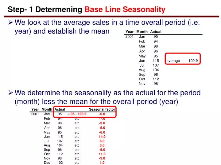
Step- 1 Determening Base Line Seasonality. We look at the average sales in a time overall period (i.e. year) and establish the mean We determine the seasonality as the actual for the period (month) less the mean for the overall period (year).

E N D
Step- 1 Determening Base Line Seasonality We look at the average sales in a time overall period (i.e. year) and establish the mean We determine the seasonality as the actual for the period (month) less the mean for the overall period (year)
A STEP BY STEP PROCESS FOR ADVANCED FORECASTING by Dr. Bjarne Berg
However, Gamma is the Seasonality Changes Gamma is the term use to see if there are changes in the seasonality In short, we may have 14 more items sold in July but this is also growing at 4 items each year. For example, In July 2001 we have sales of 115 items. This is 14 items more than the avarage for the other months of the year. But what if in July 2002 it increases to 118 items (+4) and to in July 2003 to 122 items (+4)? - We then say that the Gamma is = + 4
Step- 2 The First Base Line Forecast For the last period (month) of the overall period (year), we create the first baseline forecast. This is simply the Actual sale, less the seasonal factor. In our example it is 102 less 1 = 101
Step- 3 The First Trend factor is zero In the last period (month) of the overall period (year), we have no trends in our forecast yet. We simply flag it as “zero”. Later we will use a term called “Beta” to calculate this (more on this later)
Step- 4 The Overall long-term trend - Alpha Alpha looks at the ‘big picture’. It is a number from 0 to 1 and is used in relations to trends, seasonal factors and previous forecasts. First, we use Alpha to look at the seasonal change. In our example alpha is 0.5, so we get: 0.5*(actual – seasonal factor same period last year) or: 0.5 * (104 - (-6)) = 55 Second, we use the ‘opposite’ of Alpha to look at the base level and prior perod trend. So we get: (1-alpha) * (base level prior period plus seasonal factor last period) or: (1- 0.5) * (101 + 0) = 50.5 We add them together and get the Base level forecast for the current period 55 + 50.5 = 105.5
Step- 5 Finding the Trend factor – we call it Beta Remember that in the last period for the first year, we had no trends in our forecast yet. We simply flagged it as “zero’ For the first forecast for 2002 we introduce the term ‘beta’. This is long-term ‘hidden’ trends in our data. Beta is normally expressed in a number from 0.0 to 1.0, but can exceed this. In our example, we use a long-term beta of 0.25.
Step- 6 Beta is Used to Find trend number for a period Beta is calculated in two steps: First, we look at the base-level forecast for January 2002 and compare it to prior period (Dec. 2001): 105.5 -101 = 4.5 We multiply this with Beta: 4.5 *0.25 = 1.13 Second, we take the ‘opposite’ of beta, caluculated as 1- beta or: 1 - 0.25 = 0.75 We use this to look at the trend prior period: 0.75 * 0 = 0.00 Third, We add this together and find the trend value for the period: 1.13 + 0.00 = 1.13
Step- 7 Bringing together the Real Forecast So far we only created a trend, base line forecast and seasonality adjustments. Now we will create the actual forecast based on all these factors. We simply add these together Baseline forecast 105.50 + Trend 1.13 + Seasonal factor - 6.00 100.63
Step-8 Crating a Forecast for all periods we have data for We can now click and drag the formulas and create a forecast based for all periods we have actual data for. We will see how good our forecasting model is. Is our alpha of 0.5 the best? Is our beta of 0.25 the best? Is our gamma of 2.00 the best? In our example we have 10 years of data to test the forecasting model against
Step- 9 Examining the forecasting model visually We graph our forecast and see how our forecast is fitting the actual data Ledger: The Blue line is actual sales for 120 months The Red line if our forecast
Step- 10 Examining the model – Mean Square Error (MSE) We now calculate the MSE by: First, Sum the (The forecasted value – the actual value)2 for all forecasts. I.e. Jan 2002 = (100.63 – 104)2 =11.357 + Feb 2002 = (101 – 100)2 = 1.000 …. Second, Divide the sum by number of periods in the forecast (nine years of 12 months) = 108 MSE for our example is now 193.6 Our goal is to reduce the MSE to as small as possible by changing the alpha, beta and gamma
Step- 11 How good is the Forecast Model – MAPE MAPE is the ‘Mean Absolute Percent Error’. MAPE for each forecasted period is calculated as: [ 100 ] * [ actual value – forecast value ] Number or periods actual value I.e.: For January 2001: (100/108) * ((104-100.6)/104)) = 0.0300
Our MAPE, MSE, Alpha, Beta and Gamma Using the Excel function “goal” seek, we can find the best setting for Alpha, Beta and Gamma. First, let us try the beta MAPE Dropped to 6.14%
Our MAPE, MSE, Alpha, Beta and Gamma Now, let us try the Alpha Now let us go for Gamma MAPE Dropped to 0.06% Gamma is zero!
Data fits perfectly!!! The forecast data fits almost perfectly our real data for 10 years, and we know alpha, beta, and gamma All this is used to forecast the data for 2011 with a very high degree of accuracy!!
Other forecasting techniques Last months demand Average for the previous year Rolling average (i.e. 12 months) Gut-feeling (very popular) Simple Regression Exponential smoothing