Download
1 / 39
430 likes | 457 Views
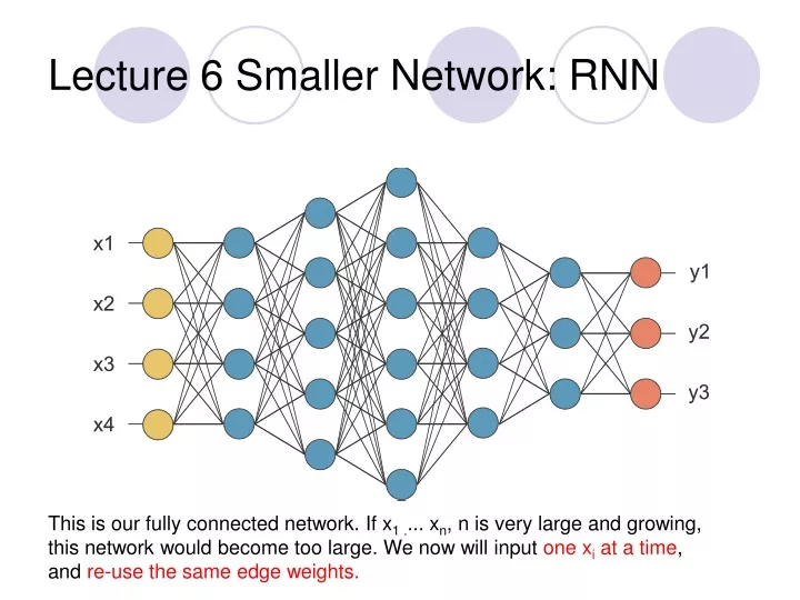
Lecture 6 Smaller Network: RNN. This is our fully connected network. If x 1 . ... x n , n is very large and growing, this network would become too large. We now will input one x i at a time , and re-use the same edge weights. Recurrent Neural Network. How does RNN reduce complexity?.

E N D
Lecture 6 Smaller Network: RNN This is our fully connected network. If x1 .... xn, n is very large and growing, this network would become too large. We now will input one xi at a time, and re-use the same edge weights.
How does RNN reduce complexity? • Given function f: h’,y=f(h,x) h and h’ are vectors with the same dimension y1 y2 y3 h0 f h1 f f h2 h3 …… x1 x2 x3 No matter how long the input/output sequence is, we only need one function f. If f’s are different, then it becomes a feedforward NN. This may be treated as another compression from fully connected network.
Deep RNN h’,y = f1(h,x), g’,z = f2(g,y) … … … z1 z2 z3 g0 f2 g1 f2 f2 g2 g3 …… y1 y2 y3 h0 f1 h1 f1 f1 h2 h3 …… x1 x2 x3
Bidirectional RNN y,h=f1(x,h) z,g = f2(g,x) x1 x2 x3 g0 f2 g1 f2 f2 g2 g3 z1 z2 z3 p1 p2 p3 f3 f3 f3 p=f3(y,z) y1 y2 y3 h0 f1 h1 f1 f1 h2 h3 x1 x2 x3
Pyramid RNN Significantly speed up training • Reducing the number of time steps Bidirectional RNN W. Chan, N. Jaitly, Q. Le and O. Vinyals, “Listen, attend and spell: A neural network for large vocabulary conversational speech recognition,”ICASSP, 2016
Wi x y Naïve RNN h f h' x h' Wh h y Wo h’ Note, y is computed from h’ softmax We have ignored the bias
Problems with naive RNN • When dealing with a time series, it tends to forget old information. When there is a distant relationship of unknown length, we wish to have a “memory” to it. • Vanishing gradient problem.
The sigmoid layer outputs numbers between 0-1 determine how much each component should be let through. Pink X gate is point-wise multiplication.
LSTM Output gate Controls what goes into output This sigmoid gate determines how much information goes thru This decides what info Is to add to the cell state Ct-1 ht-1 Forget input gate gate The core idea is this cell state Ct, it is changed slowly, with only minor linear interactions. It is very easy for information to flow along it unchanged. Why sigmoid or tanh: Sigmoid: 0,1 gating as switch. Vanishing gradient problem in LSTM is handled already. ReLU replaces tanh ok?
it decides what component is to be updated. C’t provides change contents Updating the cell state Decide what part of the cell state to output
Peephole LSTM Allows “peeping into the memory”
Naïve RNN vs LSTM yt LSTM ct yt ct-1 Naïve RNN ht ht ht-1 ht-1 xt xt c changes slowly ct is ct-1 added by something h changes faster ht and ht-1 can be very different
These 4 matrix computation should be done concurrently. W z zi Wi = σ( ) Controls forget gate Controls input gate Updating information Controls Output gate Wf zf = σ( ) z zf zi zo xt xt xt xt ht-1 ht-1 ht-1 ht-1 zo Wo = σ( ) ht-1 xt ct-1 Information flow of LSTM
W z =tanh( ) ct-1 diagonal obtained by the same way “peephole” z zf zi zo xt ht-1 zi zo zf Information flow of LSTM ht-1 xt ct-1
Element-wise multiply yt ct = zf ct-1 + ziz tanh ht = zo tanh(ct) yt = σ(W’ ht) z zf zi zo ht xt ht-1 ct-1 ct Information flow of LSTM
LSTM information flow yt+1 yt tanh tanh z zf zi zo z zf zi zo ht+1 ht xt+1 ht-1 xt ct-1 ct+1 ct Information flow of LSTM
LSTM GRU – gated recurrent unit (more compression) reset gate Update gate It combines the forget and input into a single update gate. It also merges the cell state and hidden state. This is simpler than LSTM. There are many other variants too. X,*: element-wise multiply
GRUs also takes xt and ht-1 as inputs. They perform some calculations and then pass along ht. What makes them different from LSTMs is that GRUs don't need the cell layer to pass values along. The calculations within each iteration insure that the ht values being passed along either retain a high amount of old information or are jump-started with a high amount of new information.
Feed-forward vs Recurrent Network 1. Feedforward network does not have input at each step 2. Feedforward network has different parameters for each layer x f1 a1 f2 a2 f3 a3 f4 y t is layer at = ft(at-1) = σ(Wtat-1 + bt) h0 f h1 f h2 f h3 f g y4 x3 x4 x1 x2 t is time step at= f(at-1, xt) = σ(Wh at-1 + Wixt + bi) We will turn the recurrent network 90 degrees.
at-1 yt at-1 No input xt at each step ht-1 at No output yt at each step ht 1- at-1 is the output of the (t-1)-th layer reset update at is the output of the t-th layer r z h' No reset gate ht-1 xt xt
h’=σ(Wat-1) Highway Network z=σ(W’at-1) at = z at-1 + (1-z) h • Highway Network • Residual Network at at + at-1 z controls red arrow h’ h’ Gate controller copy copy at-1 at-1 Deep Residual Learning for Image Recognition http://arxiv.org/abs/1512.03385 Training Very Deep Networks https://arxiv.org/pdf/1507.06228v2.pdf
output layer output layer output layer Highway Network automatically determines the layers needed! Input layer Input layer Input layer
Grid LSTM Memory for both time and depth depth y c’ Grid LSTM LSTM c’ c c h’ h’ h h a b x a’ b’ time
Grid LSTM tanh c’ Grid LSTM c h’ h zf zi z zo a b a’ b’ c a a' c' You can generalize this to 3D, and more. h' b' h b
Chat with context M: Hi M: Hello U: Hi M: Hi U: Hi M: Hello Serban, Iulian V., Alessandro Sordoni, Yoshua Bengio, Aaron Courville, and Joelle Pineau, 2015 "Building End-To-End Dialogue Systems Using Generative Hierarchical Neural Network Models.
Image caption generation using attention(From CY Lee lecture) z0 is initial parameter, it is also learned A vector for each region match 0.7 filter filter filter CNN filter filter filter filter filter filter filter filter filter z0
Image Caption Generation Word 1 A vector for each region z0 Attention to a region weighted sum filter filter filter CNN filter filter filter 0.1 0.1 0.7 0.1 0.0 0.0 filter filter filter filter filter filter z1
Image Caption Generation Word 2 Word 1 A vector for each region z2 weighted sum filter filter filter CNN filter filter filter 0.8 0.2 0.0 0.0 0.0 0.0 filter filter filter filter filter filter z1 z0
Image Caption Generation Kelvin Xu, Jimmy Ba, Ryan Kiros, Kyunghyun Cho, Aaron Courville, Ruslan Salakhutdinov, Richard Zemel, Yoshua Bengio, “Show, Attend and Tell: Neural Image Caption Generation with Visual Attention”, ICML, 2015
Image Caption Generation Kelvin Xu, Jimmy Ba, Ryan Kiros, Kyunghyun Cho, Aaron Courville, Ruslan Salakhutdinov, Richard Zemel, Yoshua Bengio, “Show, Attend and Tell: Neural Image Caption Generation with Visual Attention”, ICML, 2015
* Possible project? Li Yao, Atousa Torabi, Kyunghyun Cho, Nicolas Ballas, Christopher Pal, Hugo Larochelle, Aaron Courville, “Describing Videos by Exploiting Temporal Structure”, ICCV, 2015