Download
1 / 34
340 likes | 347 Views
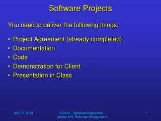
Estimation for Software Projects. Software Project Planning. The overall goal of project planning is to establish a pragmatic strategy for controlling, tracking, and monitoring a complex technical project. Why? So the end result gets done on time, with quality!. Project Planning Task Set-I.

E N D
Software Project Planning The overall goal of project planning is to establish a pragmatic strategy for controlling, tracking, and monitoring a complex technical project. Why? So the end result gets done on time, with quality!
Project Planning Task Set-I • Establish project scope • Determine feasibility • Analyze risks • Define required resources • Determine require human resources • Define reusable software resources • Identify environmental resources
Project Planning Task Set-II • Estimate cost and effort • Decompose the problem • Develop two or more estimates using size, function points, process tasks or use-cases • Reconcile the estimates • Develop a project schedule • Establish a meaningful task set • Define a task network • Use scheduling tools to develop a timeline chart • Define schedule tracking mechanisms
Estimation • Estimation of resources, cost, and schedule for a software engineering effort requires • experience • access to good historical information (metrics) • the courage to commit to quantitative predictions when qualitative information is all that exists • Estimation carries inherent risk and this risk leads to uncertainty
Software Project Plan ? Project Scope Estimates Risks Schedule Control strategy Software Project Plan
To Understand Scope ... • Understand the customers needs • understand the business context • understand the project boundaries • understand the customer’s motivation • understand the likely paths for change • understand that ... Even when you understand, nothing is guaranteed!
What is Scope? • Software scopedescribes • The functions and features that are to be delivered to end-users • The data that are input and output • The performance, constraints, interfaces, and reliability that bound the system. • Scope is defined using one of two techniques: • A narrative description of software scope is developed after communication with all stakeholders. • A set of use-cases is developed by end-users.
Project Estimation • Project scope must be understood • Elaboration (decomposition) is necessary • Historical metrics are very helpful • At least two different techniques should be used • Uncertainty is inherent in the process
Estimation Techniques • Past (similar) project experience • Conventional estimation techniques • task breakdown and effort estimates • size (e.g., FP) estimates • Empirical models • Automated tools
Estimation Accuracy • Based on … • the degree to which the planner has properly estimated the size of the product to be built • the degree to which the project plan reflects the abilities of the software team • the stability of product requirements and the environment that supports the software engineering effort.
Functional Decomposition Statement of Scope functional decomposition Perform a Grammatical “parse”
Conventional Methods:LOC/FP Approach • Compute LOC/FP using estimates of information domain values • Use historical data to build estimates for the project
Example: LOC Approach Average productivity for systems of this type = 620 LOC/pm. Burdened labor rate =$8000 per month, the cost per line of code is approximately $13. Based on the LOC estimate and the historical productivity data, the total estimated project cost is $431,000 and the estimated effort is 54 person-months.
Example: FP Approach The estimated number of FP is derived: FPestimated = count-total 3 [0.65 + 0.01 x S(Fi)] FPestimated = 375 organizational average productivity = 6.5 FP/pm. burdened labor rate = $8000 per month, approximately $1230/FP. Based on the FP estimate and the historical productivity data, total estimated project cost is $461,000 and estimated effort is 58 person-months.
Example: FP Approach Complexity adjustment factor 1.17 The estimated number of FP is derived: FPestimated = count-total X [0.65 + 0.01 X S(Fi)] FPestimated =320 X 1.17 FPestimated = 375 organizational average productivity = 6.5 FP/pm. burdened labor rate = $8000 per month, approximately $1230/FP. Based on the FP estimate and the historical productivity data, total estimated project cost is $461,000 and estimated effort is 58 person-months.
Process-Based Estimation Obtained from “process framework” framework activities application functions Effort required to accomplish each framework activity for each application function
Process-Based Estimation Example Based on an average burdened labor rate of $8,000 per month, the total estimated project cost is $368,000 and the estimated effort is 46 person-months.
Empirical Estimation Models The Structure of Estimation Models E = A + B x (ev)C • where • A, B, and C are empirically derived constants, • E is effort in person-months, • ev is the estimation variable (either LOC or FP).
Empirical Estimation Models • Among the many LOC-oriented estimation models proposed in the literature are • Walston-Felix model E = 5.2 x (KLOC)0.91 • Bailey-Basili model E = 5.5 + 0.73 x (KLOC)1.1 • Boehm simple model E = 3.2 x (KLOC)1.05 • Doty model for KLOC > 9 E = 5.288 x (KLOC)1.047 • FP-oriented models • Albrecht and Gaffney model E = -13.39 + 0.0545 FP • Kemerer model E = 60.62 x 7.728 x 10-8FP3 • Matson, Barnett and Mellichamp model E = 585.7 + 15.12 FP
COnstructive COst MOdel.COCOMO-II ( Successor of COCOMO - introduced in 80s) • COCOMO II is actually a hierarchy of estimation models that address the following areas: • Application composition model. Used during the early stages of software engineering, when prototyping of user interfaces, consideration of software and system interaction, assessment of performance, and evaluation of technology maturity are paramount. • Early design stage model. Used once requirements have been stabilized and basic software architecture has been established. • Post-architecture-stage model. Used during the construction of the software.
COCOMO-II • Sizing information • object points, • function points, • lines of source code. • The object point is an indirect software measure (like FP) that is computed using counts of the number of • screens (at the user interface), • reports, • components likely to be required to build the application. • Each object instance (e.g., a screen or report) is classified into one of three complexity levels (simple, medium, or difficult) • Complexity is a function of the number and source of the client and server data tables that are required to generate the screen or report and the number of views or sections presented as part of the screen or report.
COCOMO-II • Once complexity is determined, the number of screens, reports, and components are weighted according to Table • The object point count is determined by multiplying the original number of object instances by the weighting factor.
COCOMO-II • When component-based development or general software reuse is to be applied, the percent of reuse (%reuse) is estimated and the object point count is adjusted: NOP = (object points) x [(100 - %reuse) / 100] where NOP is defined as new object points • Now estimated effort = NOP/PROD Where PROD ( Productivity Rate ) may be derived from
The Software Equation • A dynamic multivariable model • E = [LOC x B0.333/P]3 x (1/t4) • where • E = effort in person-months or person-years • t = project duration in months or years • B = “special skills factor” • P = “productivity parameter” that reflects: • Overall process maturity and management practices • The extent to which good software engineering practices are used • The level of programming languages used • The state of the software environment • The skills and experience of the software team • The complexity of the application
Estimation for OO Projects-I • Develop estimates using effort decomposition, FP analysis, and any other method that is applicable for conventional applications. • Using object-oriented requirements modeling develop use-cases and determine a count. • From the analysis model, determine the number of key classes • Categorize the type of interface for the application and develop a multiplier for support classes: Interface type Multiplier No GUI 2.0 Text-based user interface 2.25 GUI 2.5 Complex GUI 3.0
Estimation for OO Projects-II • Multiply the number of key classes (step 3) by the multiplier to obtain an estimate for the number of support classes. • Multiply the total number of classes (key + support) by the average number of work-units per class. Lorenz and Kidd suggest 15 to 20 person-days per class. • Cross check the class-based estimate by multiplying the average number of work-units per use-case
Estimation for Agile Projects • Each user scenario (a mini-use-case) is considered separately for estimation purposes. • The scenario is decomposed into the set of software engineering tasks that will be required to develop it. • Each task is estimated separately. Note: estimation can be based on historical data, an empirical model, or “experience.” • Alternatively, the ‘volume’ of the scenario can be estimated in LOC, FP or some other volume-oriented measure (e.g., use-case count). • Estimates for each task are summed to create an estimate for the scenario. • Alternatively, the volume estimate for the scenario is translated into effort using historical data. • The effort estimates for all scenarios that are to be implemented for a given software increment are summed to develop the effort estimate for the increment.
Computing Expected Cost expected cost = (path probability) x (estimated path cost) i i For example, the expected cost to build is: similarly,
Estimation with Use-Cases User interface subsystem ( UICF ) Engineering subsystem group ( 2DGA+3DGA+DAM ) Infrastructure subsystem group ( CGDF+PCF ) Using 620 LOC/pm as the average productivity for systems of this type and a burdened labor rate of $8000 per month, the cost per line of code is approximately $13. Based on the use-case estimate and the historical productivity data, the total estimated project cost is $552,000 and the estimated effort is 68 person-months.