Download
1 / 38
380 likes | 438 Views
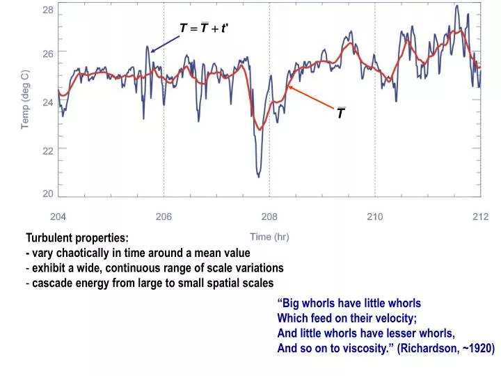
Turbulent properties: - vary chaotically in time around a mean value exhibit a wide, continuous range of scale variations cascade energy from large to small spatial scales. “Big whorls have little whorls Which feed on their velocity; And little whorls have lesser whorls,

E N D
Turbulent properties: • - vary chaotically in time around a mean value • exhibit a wide, continuous range of scale variations • cascade energy from large to small spatial scales “Big whorls have little whorls Which feed on their velocity; And little whorls have lesser whorls, And so on to viscosity.” (Richardson, ~1920)
- Use these properties of turbulent flows in the Navier Stokes equations • The only terms that have products of fluctuations are the advection terms • All other terms remain the same, e.g.,
0 are the Reynolds stresses arise from advective (non-linear or inertial) terms
Turbulent Kinetic Energy (TKE) An equation to describe TKE is obtained by multiplying the momentum equation for turbulent flow times the flow itself (scalar product) Total flow = Mean plus turbulent parts = Same for a scalar:
Multiplying turbulent flow times ui and dropping the primes fluctuating strain rate Turbulent Kinetic Energy (TKE) Equation Total changes of TKE Transport of TKE Shear Production Buoyancy Production Viscous Dissipation Transport of TKE. Has a flux divergence form and represents spatial transport of TKE. The first two terms are transport of turbulence by turbulence itself: pressure fluctuations (waves) and turbulent transport by eddies; the third term is viscous transport
interaction of Reynolds stresses with mean shear; represents gain of TKE represents gain or loss of TKE, depending on covariance of density and w fluctuations represents loss of TKE
In many ocean applications, the TKE balance is approximated as:
The rate of energy transfer to smaller scales can be estimated from scaling: u velocity of the eddies containing energy l is the length scale of those eddies u2 kinetic energy of eddies l / u turnover time u2/ (l /u )rate of energy transfer = u3 / l ~ At any intermediate scale l, But at the smallest scales LK, Kolmogorov length scale so that Typically, The largest scales of turbulent motion (energy containing scales) are set by geometry: - depth of channel - distance from boundary
Vertical Shears (vertical gradients) Shear production from bottom stress z u bottom
z W Vertical Shears (vertical gradients) u Shear production from wind stress
Vertical Shears (vertical gradients) Shear production from internal stresses z u1 u2 Flux of momentum from regions of fast flow to regions of slow flow
Near the bottom Bottom stress: Parameterizations and representations of Shear Production Law of the wall
Data from Ponce de Leon Inlet Florida FloridaIntracoastal Waterway
(Monismith’s Lectures) Law of the wall may be widely applicable
(Monismith’s Lectures) Ralph Obtained from velocity profiles and best fitting them to the values of z0 and u*
Shear Production from Reynolds’ stresses Mixing of property S Mixing of momentum Munk & Anderson (1948, J. Mar. Res., 7, 276) Pacanowski & Philander (1981, J. Phys. Oceanogr., 11, 1443)
With ADCP: and θ is the angle of ADCP’s transducers -- 20º Lohrmann et al. (1990, J. Oc. Atmos. Tech., 7, 19)
Souza et al. (2004, Geophys. Res. Lett., 31, L20309) Day of the year (2002)
S2 > S1 S1, T1 T2 > T1 S2, T2 Buoyancy Production from Cooling and Double Diffusion
Layering Experiment http://www.phys.ocean.dal.ca/programs/doubdiff/labdemos.html
Data from the Arctic From Kelley et al. (2002, The Diffusive Regime of Double-Diffusive Convection)
Dissipation from strain in the flow (m2/s3) (Jennifer MacKinnon’s webpage)
Production of TKE From: Rippeth et al. (2003, JPO, 1889) Dissipation of TKE
Example of Spectrum – Electromagnetic Spectrum http://praxis.pha.jhu.edu/science/emspec.html
Other ways to determine dissipation (indirectly) Kolmogorov’s K-5/3 law S (m3 s-2) Wave number K (m-1)
P equilibrium range inertial dissipating range Kolmogorov’s K-5/3 law (Monismith’s Lectures)
Kolmogorov’s K-5/3 law -- one of the most important results of turbulence theory (Monismith’s Lectures)
Stratification kills turbulence In stratified flow, buoyancy tends to: i) inhibit range of scales in the subinertial range ii) “kill” the turbulence
(responsible for dissipation of TKE) At intermediate scales --Inertial subrange – transfer of energy by inertial forces (Monismith’s Lectures)
Other ways to determine dissipation (indirectly) (Monismith’s Lectures)