Download
1 / 30
300 likes | 445 Views
Envisioning Information Lecture 14 – Scientific Visualization Scalar 3D Data – Volume Rendering. Ken Brodlie kwb@comp.leeds.ac.uk. Volume Rendering. This is a quite different mapping technique for visualization of 3D scalar data (compared with isosurfacing)

E N D
Envisioning Information Lecture 14 – Scientific Visualization Scalar 3D Data – Volume Rendering Ken Brodlie kwb@comp.leeds.ac.uk ENV 2006
Volume Rendering • This is a quite different mapping technique for visualization of 3D scalar data (compared with isosurfacing) • Aims to relate volume to a partially opaquegel material - colour and opacity at a point depending on the scalar value • By controlling the opacity, we can: • EITHER show surfaces through setting opacity to 0 or 1 • OR see both exterior and interior regions by grading the opacity from 0 to 1 [Note: opacity = 1 - transparency] ENV 2006
Example - Forest Fire From Numerical Model of Forest Fire, NCAR, USA ENV 2006
Medical Imaging • Major application area is medical imaging • Different scanning techniques include: • CT (Computed Tomography) • MRI (Magnetic Resonance Imaging) • SPECT (Single Photon Emission Computed Tomography) • Three-dimensional images constructed from multiple 2D slices Slice Scanners give average value for a region - rather than value at a point Interslice gap Slice ENV 2006
Examples of Brain Scans Magnetic Resonance Imaging Computerized Tomography SPECT ENV 2006
Example - Medical Imaging Rendered by VolPack software CT scan data 256x256x226 ENV 2006
Opacity a 1 0 CT value fsoft_tissue Data Classification – Assigning Opacity to CT data • CT will identify fat, soft tissue and bone • Each will have known absorption levels, say ffat, fsoft_tissue, fbone This transferfunction will highlight soft tissue ENV 2006
Opacity a 1 0 CT value fsoft_tissue Data Classificatiion – Assigning Opacity to CT Data • To show all types of tissue, we assign opacities to each type and linearly interpolate between them ffat fbone ENV 2006
Data Classification – Constructing the Gel – CT Data opacity This is known as opacity transfer function 1.0 CT number 0.0 (f) In practice, the boundaries between materials are of key importance - hence a two-stage algorithm used: (i) Calculate as above (ii) Scale by gradient of function to highlight boundaries * = |grad f | grad f = [df/dx,df/dy,df/dz] ? So what is opacity in homogeneous areas ? ENV 2006
Data Classification – Constructing the Gel – CT Data • Colour classification is done similarly Known as colour transfer function white red yellow CT number Soft Tissue Air Fat Bone ENV 2006
red (1,0,0) blue (0,0,1) temperature Data Classification – Constructing the Gel – Temperature Data • Volume rendering is also useful for other data - eg CFD temperature • Opacity transfer function: possibly increase with temperature • Colour transfer function: ENV 2006
The GenerateColormap tool in IRIS Explorer can be used to assign colour and transparency to data Make sure you know how to save colourmaps from one session to another Data Classification in IRIS Explorer ENV 2006
Example Storm cloud data rendered by IRIS Explorer – Isosurface & volume rendering ENV 2006
Rendering the Volume • There are two major techniques: • Ray casting • Texture mapping ENV 2006
Ray Casting to Render the Volume 1 Assign colour and opacity to data values • Classification process assigns gel colour to the original data 2 Apply light to volume • Lighting model will give the light reflected to the viewer at any point in volume - if we know the normal • Imagine an isosurface shell through each data point - surface normal is provided by gradient vector (remember from isosurfacing!) • Thus we get colour reflected at each data point ENV 2006
Casting the Rays and Taking Samples • 3. For each pixel in image • a) cast ray from eye through pixel into volume, taking samples at regular unit intervals • b) measure colour reflected at each sample in direction of ray • c) composite colour from all samples along ray, taking into account the opacity of gel it passes through - en route to the eye data volume ray eye point exit point image plane sample points one unit apart (colour and opacity by interpolation) entry point ENV 2006
Compositing the Samples Along the Ray – First Sample opaque background, emitting I0 I0 I* eye point Intensity - I1 Opacity - Imagine block of gel, one unit wide around sample point I* = I0 (1 - ) + I1 ENV 2006
Compositing the Samples along the Ray – Two Samples opaque background I** I* I0 eye point Intensity - I2 Opacity - 2 Intensity - I1 Opacity - I* = I0 (1 - ) + I1 ... from previous slide I** = I* (1 - 2) + I22 = I0 (1 - 1)(1 - 2) + I11(1 - 2) + I22 ENV 2006
Compositing the Samples along a Ray • The process continues for all samples, yielding a final intensity, or colour, for the ray - and this is assigned to the pixel • try it for a third sample, then you should be able to deduce a general formula I = Sni=0 Iii Pnj=i+1(1 - j) • Note that if one compositing step is done for each ray in turn, then the next step, and so on, the image will be created in a sweep from back to front, showing all the data (even behind opaque parts) ENV 2006
Front to Back Compositing Compositing can also work front-to-back: I* eye point I* = n In - cumulative opacity * = n Intensity In Opacity n I** eye point I** = I* + (1 - *)n-1In-1 ** = * + (1-*)n-1 Intensity In Opacity n Intensity In-1 Opacity n-1 ENV 2006
Front-to-Back Compositing – Early Termination • The advantage of front-to-back compositing is that we can stop the process if the accumulated opacity reaches 1.0 - no point in going further • Again, you should be able to deduce the general formula if you look at three samples • can you show that front-to-back and back-to-front compositing give the same answer? ENV 2006
When performance rather than accuracy is the goal, we can avoid compositing altogether and approximate I by maximum intensity along ray MIP : Maximum Intensity Projection Often used in angiography... Maximum Intensity Projection ENV 2006
Texture-based Volume Rendering • Volume rendering by ray casting is time-consuming • one ray per pixel • each ray involves tracking through volume calculating samples, and then compositing • different for each viewpoint • Alternative approach - using texture maps - can exploit graphics hardware ENV 2006
Modern graphics hardware includes facility to draw a textured polygon The texture is an image with red, green, blue and alpha components… … this is used in computer graphics to avoid constructing complex geometric models Texture Mapping … and we can exploit this in volume rendering ENV 2006
Texture-based Volume Rendering • Draw from back-to-front a set of rectangles • first rectangle drawn as an area of coloured pixels, with associated opacity, as determined by transfer function and interpolation - and merged with background in a compositing operation (supported by hardware) • successive rectangles drawn on top ENV 2006
For a given viewing direction, we would need to select slices perpendicular to this direction This requires interpolation to get the values on the slices Until recently this has only been possible with expensive graphics boards 3D Texture-based Volume Rendering volume image plane 3D texture mapping ENV 2006
Comparison of Ray Casting and Texture Approaches Ray casting Texture-based Texture-based Ray casting http://www.cora.nwra.com/Ogle/ http://vg.swan.ac.uk/vlib http://www.amiravis.com ENV 2006
Close Up Ogle: texture-based Vlib: ray casting ENV 2006
Another commonly used method is splatting Fuzzy balls around each voxel projected on to image plane Composited in the image plane VolumeToGeom in IRIS Explorer Splatting ENV 2006
Classic paper: M. Levoy. Efficient ray tracing of volume data. ACM Trans Graphics, Vol 9, 3, pp245-261, 1990 Recent work: Ray casting: S. Grimm, S. Bruckner, A. Kanitsar, E. Groller.Memory efficient acceleration structures and techniques for CPU-based volume raycasting of large data. In Proceedings of the IEEE Symposium on Volume Visualization and Graphics 2004 (Oct. 2004), pp. 1-8. Texture-based: K. Engel et al, Real-time volume graphics. Tutorial 28 in SIGGRAPH2004, See <http://www.vrvis.at/via/resources/course-volgraphics-2004/> References ENV 2006