Download
1 / 23
240 likes | 457 Views
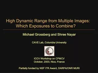
High Dynamic Range from Multiple Images: Which Exposures to Combine?. Michael Grossberg and Shree Nayar CAVE Lab, Columbia University ICCV Workshop on CPMCV October, 2003, Nice, France Partially funded by NSF ITR Award, DARPA/ONR MURI. +. Combining Different Exposures.

E N D
High Dynamic Range from Multiple Images: Which Exposures to Combine? Michael Grossberg and Shree Nayar CAVE Lab, Columbia University ICCV Workshop on CPMCV October, 2003, Nice, France Partially funded by NSF ITR Award, DARPA/ONR MURI
+ Combining Different Exposures Low Dynamic Range Exposures Combination Yields High Dynamic Range [Ginosar and Zeevi, 88, Madden, 93, Mann and Picard, 95, Debevec and Malik, 97, Mitsunaga and Nayar, 99]
0 255 Camera Response Image Intensity f B The Camera Response Linear Function (Optical Attenuation) Image Irradiance Scene Radiance E L s
Measured Irradiance Levels From Response To Measured Irradiance Levels Response Function f Brightness Levels B Irradiance E
Where do you want your bits? Response Function f Coarse quantization Brightness B High Dynamic Range Irradiance E Response Function f Fine quantization Brightness B Low Dynamic Range Irradiance E
+ + Capture Irradiance Uniformly Effective Camera from Multiple Exposures Goal Acquired Images Image from Effective Camera Capture High Dynamic Range
Flexible Dynamic Range Imaging: • Can we create an effective camera with a desired response? • How many exposures are needed? • Which exposures to acquire? • How to combine the acquired images?
3 2 1 0 Sum 0 E1 E2 E3 3 2 1 0 0 E1 /e1 E2 /e2 E3 /e3 6 5 4 3 2 1 0 ^ ^ ^ ^ ^ ^ 0 E1 E2 E3 E4 E5 E6 Irradiance Levels From Multiple Exposures f(E) Exposuree1 = 1 Irradiance E f(e2E) Exposuree2 h(E) Effective Camera
Response of the Effective Camera Effective Response Number of exposures Camera Response Exposures Irradiance Theorem: The sum of a set of images of a scene taken at different exposures includes all the information in the individual exposures.
~ h Camera Response Emulation • How can we tell if h emulates g well? Naïve answer:| h – g | < e Emulated Response depends on: h f , e = (e1, … ,en) Brightness Levels B g Desired Response Irradiance E Level spacing characterizes similarity
Smaller Derivatives Sparse Spacing Measured Irradiance Levels How Response Determines Level Spacing h Observation: The derivativedetermines the distances between levels. Larger Derivative Brightness Levels B Dense Spacing Irradiance E
h g Brightness B 0, 1, otherwise w=0 w=1 Irradiance E The Objective Function Spacing Based Comparison: Number of Exposures Exposure Values Desired Response Effective Response Weight Weight prevents penalizing success:
Which Exposures and How Many? • For fixed n, find minimizing exposure values e • Choose min n such that error within tolerance • Method: Exhaustive search • Objective function not continuous • Only need to search actual settings • Offline build table of exposures
Effective Camera Number of Exposures Exposure Values 1 2 3 4 5 6 1 1.003 2 Linear 1 1.003 2.985 3 1 1.015 1.019 3.672 4 5 1 1.003 1.007 1.166 4.975 1 1.003 1.007 1.031 1.078 5.636 6 1 3.094 2 Gamma = 1/2 3 1 1.003 5.146 1 1.003 3.019 11.23 4 1 1.003 1.006 5.049 18.56 5 6 1 1.003 1.006 2.866 8.564 33.7 1 20.24 2 Constant contrast (log) 1 9.91 88.38 3 1 4.689 37.23 280 4 5 1 4.831 29.18 144.9 763.5 6 1 3.979 16.01 64.22 305.4 1130 Flexible Dynamic Range Imaging
Dynamic Range High 1:16,000 Low 1:256 Desired Response Constant Contrast Dynamic Range Desired Response Linear High 1:16,000 Gamma 1/2 Constant Contrast Medium 1:1,000 Linear Low 1:256 Gamma 1/2 Effective Camera Number of Exposures Exposure Values 1 2 3 4 5 6 1 1.003 2 Linear 1 1.003 2.985 3 1 1.015 1.019 3.672 4 5 1 1.003 1.007 1.166 4.975 1 1.003 1.007 1.031 1.078 5.636 6 1 3.094 2 Gamma = 1/2 3 1 1.003 5.146 1 1.003 3.019 11.23 4 1 1.003 1.006 5.049 18.56 5 6 1 1.003 1.006 2.866 8.564 33.7 1 20.24 2 Constant contrast (log) 1 9.91 88.38 3 1 4.689 37.23 280 4 5 1 4.831 29.18 144.9 763.5 6 1 3.979 16.01 64.22 305.4 1130 Flexible Dynamic Range Imaging
Baseline Exposure Values • Typically exposures are doubled • Baseline: Combine the exposures e =(1,2,4) [Ginosar and Zeevi, 88, Madden, 93, Mann and Picard, 95, Debevec and Malik, 97, Mitsunaga and Nayar, 99]
1.0 0.8 0.6 0.4 0.2 0.0 0.0 0.2 0.4 0.6 0.8 1.0 4-bit real camera 1.0 BaselineResponse (1,2,4) Baseline Response (1,2,4) 0.8 0.6 BrightnessB Brightness B Desired Response 0.4 Desired Response 0.2 Computed Response Computed Response (1, 1.05, 1.11) (1, 1.003, 2.985) 0.0 0.0 0.2 0.4 0.6 0.8 1.0 IrradianceE IrradianceE Increased Dynamic Range Linear Camera • Real Camera: f linear • Desired Camera: g linear (greater dynamic range) Brightness Brightness 8-bit real camera
High Dynamic Range Linear Camera From baseline exposures (1,2,4) From computed exposures (1,1.05,1.11) Linear Camera: Synthetic Ramp Image
Baseline Exposures (1,2,4) Ground Truth (HDR image) Linear Camera: Image of Cloth Computed Exposures (1,1.05,1.11)
3 Exposures 5 Exposures 1.0 1.0 Desired Response Desired Response 0.8 0.8 0.6 Baseline Response (1,2,4) 0.6 Baseline Response BrightnessB BrightnessB 0.4 0.4 0.2 Computed Response (1,9.91,88.38) Computed Response 0.2 0.0 0.0 1.0 0.0 0.2 0.4 0.6 0.8 1.0 0.0 0.2 0.4 0.6 0.8 IrradianceE IrradianceE Constant Contrast from Linear Cameras • Real Camera: f linear • Desired Camera: g log response (constant contrast)
Constant Contrast : Image of Tiles Baseline Exposures Computed Exposures
Baseline Input Exposures Computed Input Exposures Combined Iso-brightness Combined Iso-brightness Linear Camera from Non-linear Camera • Real Camera: f non-linear (Nikon 990) • Desired Camera: g linear Brightness Brightness
Summary • Combine images using summation • Method finds number of exposures and exposure values to use • Emulation of a variety of cameras: Flexible Dynamic Range Imaging