Download

1 / 15
150 likes | 388 Views
259 Lecture 18. The Symbolic Toolbox. The Symbolic Toolbox. MATLAB has a set of built-in commands that allow us to work with functions in a fashion similar to Mathematica .

E N D
259 Lecture 18 The Symbolic Toolbox
The Symbolic Toolbox • MATLAB has a set of built-in commands that allow us to work with functions in a fashion similar to Mathematica. • Octave can also perform some of the same functionality via the “symbolic” package – we will look at this after the MATLAB features! • For more on the commands available, type “help Symbolic Toolbox”. • The commands we will look at are: • sym, syms, diff, int, simplify, pretty, subs, double, and ezplot. • For help on these commands, use the help file. • If a symbolic command has the same name as a numerical command, such as “diff”, typing “help sym/commandname” will give help on the symbolic command. • Try “help diff” and “help sym/diff”.
To define symbolic variables in MATLAB, use the “sym” command. Example 1a: Here’s how to define variables x, y, and a, and functions f(x) = x3 + 2x2 +x-1 g(x) = sin(x) h(y) = (a2-y2)/(y+1) x = sym(‘x’) y = sym(‘y’) a = sym(‘a’) f = x^3+2*x^2+x-1 g = sin(x) h = sqrt(a^2-y^2)/(y+1) Typing “pretty(h)” will make h(y) look nicer! Note that in MATLAB, “syms x y a” also worksto define symbolic variables! sym
To find the derivative of a function defined symbolically, we use the “diff” command. Example 2a: Find the following derivatives of the functions from Example 1a: f’(x), f’’(x), g’(x), h’’’(y). Also find dy/dx if y = x + x2 – x4 or y = tan(x)sin(x) -ln(x)/ex diff(f) fprime = diff(f) f2prime = diff(f,2) gprime = diff(g) h3prime = diff(h,3) pretty(h3prime) simplify(h3prime) pretty(simplify(h3prime)) diff('x + x^2 - x^4') diff('tan(x)^sin(x) -log(x)/exp(x)') pretty(ans) diff
To evaluate a symbolic function we use the command “subs”. Example 3a: For the functions defined in Example 1a, find each of the following: f(-3) f(v) where v = [1 2 4] g’(pi/4) h(1) h(1) with a = 2 h(y) with a = 2 subs(f,-3) v = [1 2 4] subs(f,v) subs(gprime,pi/4) subs(h,1) b = subs(h,1) subs(b,2) subs(h,'a',2) subs
We can plot symbolic functions with the command “ezplot”! Example 4a: Use ezplot to graph the functions f(x), g(x), g’(x), f’(x), and f’’(x) defined in Example 1a. Note that the default settings for ezplot can be changed with title, xlabel, and ylabel. The default x-interval of [-2, 2] can also be changed. ezplot(f) ezplot(f,[-1,1]) ezplot(g) ezplot(gprime,[0,2*pi]) One way to plot multiple graphs via ezplot: ezplot(f) hold on ezplot(fprime) ezplot(f2prime) title('Plot of f and it''s derivatives.') hold off ezplot
To find indefinite or definite integrals in MATLAB, we use “int”. Example 5: Find each integral: int(f) int(g,0,pi) int(h,'y',0.5,1) pretty(ans) sym(a,'positive') int(h,'y',0.5,1) pretty(ans) int(h,'a',0.5,1) int('x + x^2 - x^4') int
funtool • Finally, here’s a way to work with functions that is more “user friendly”. • Typing “funtool” brings up a function calculator in MATLAB. • funtool is a visual function calculator that manipulates and displays functions of one variable. • At startup, funtool displays graphs of a pair of functions, f(x) = x and g(x) = 1. • The graphs plot the functions over the domain [-2*pi, 2*pi]. • funtool also displays a control panel that lets you save, retrieve, redefine, combine, and transform f and g.
Symbolic Package in Octave • To perform symbolic manipulation in Octave, first we need to load the “symbolic” package. • The symbolic package, as well as other add-ons can be found here: • Octave downloads from Source Forge (both Windows and Mac OS X installers can be found here: http://octave.sourceforge.net/ • Octave Homepage: http://www.gnu.org/software/octave/ • A reference for the “symbolic” package can be found here (choose “Function Reference”): • http://octave.sourceforge.net/symbolic/index.html
Symbolic Functions in Octave • Once the “symbolic” package is installed, turn on Octave and type “pkg load all” to load all installed packages. • To enable the symbolic features in Octave, type “symbols”.
To define symbolic variables in Octave, use the “sym” command. Example 1b: Here’s how to define variables x, y, and a, and functions f(x) = x3 + 2x2 +x-1 g(x) = sin(x) h(y) = (a2-y2)/(y+1) x = sym(‘x’) y = sym(‘y’) a = sym(‘a’) f = x^3+2*x^2+x-1 g = Sin(x) h = Sqrt(a^2-y^2)/(y+1) sym in Octave
To find the derivative of a function defined symbolically in Octave, we use the “differentiate” command. Example 2b: Find the following derivatives of the functions from Example 1b: f’(x), f’’(x), g’(x), h’’’(y). Also find dy/dx if y = x + x2 – x4 or y = tan(x)sin(x) -ln(x)/ex differentiate(f,x) fprime = differentiate(f,x) f2prime = differentiate(f,x,2) gprime = differentiate(g,x) h3prime = differentiate(h,y,3) differentiate(x + x^2 - x^4,x) differentiate(Tan(x)^Sin(x) -Log(x)/Exp(x),x) diff in Octave
To evaluate a symbolic function in Octave, we use the command “subs”. Example 3b: For the functions defined in Example 1b, find each of the following: f(-3) g’(pi/4) h(1) h(1) with a = 2 h(y) with a = 2 subs(f,x,-3) subs(gprime,pi/4) subs(h,y,1) b = subs(h,y,1) subs(b,a,2) subs(h,a,2) subs in Octave
We can plot symbolic functions with the command “ezplot”! Example 4b: Use ezplot to graph the functions f(x), g(x), g’(x), f’(x), and f’’(x) defined in Example 1b. Note that the default settings for ezplot can be changed with title, xlabel, and ylabel. The default x-interval of [-2, 2] can also be changed. Recall that f = x^3+2*x^2+x-1 g = Sin(x) ezplot(‘x^3+2*x^2+x-1’) ezplot(‘x^3+2*x^2+x-1’,[-1,1]) ezplot(‘sin(x)’) ezplot(‘cos(x)’,[0,2*pi]) One way to plot multiple graphs via ezplot: ezplot(‘x^3+2*x^2+x-1’) hold on ezplot(‘3*x^2+4*x+1’) ezplot(‘6x+4’) title('Plot of f and it''s derivatives.') hold off ezplot in Octave
References Using MATLAB in Calculus by Gary Jenson MATLAB Help File 15 15