Download
1 / 10
100 likes | 213 Views
Four hipsters bump into each other in a crowed elevator and drop their identical cell phones as the elevator doors are closing. In the scramble to retrieve their phones, each one picks up a phone at random.

E N D
Four hipsters bump into each other in a crowed elevator and drop their identical cell phones as the elevator doors are closing. In the scramble to retrieve their phones, each one picks up a phone at random. We will reconsider this scenario to determine the theoretical probability of various outcomes/events The probability of a random event occurring is defined as the long-run proportion (or relative frequency) of times the event would occur if the random process that generates the event were repeated a large number of times under essentially identical conditions.
In situations where the outcomes of a random process are equally likely, the theoretical (exact) probability of each outcome can be determined by listing all of the possible outcomes and determining the proportion that corresponds to the event of interest. The list of all possible outcomes is called the sample space.
The long–run average value of a such a quantitative variable is called its expected value. The listing of possible values of a quantitative variable (its outcomes) generated by a random process, along with the probabilities for those values, is called its probability distribution. To calculate this expected value from a probability distribution: 1. Multiply each outcome by its probability 2. Add these “weighted” values over all possible outcomes outcome 1 x prob. of outcome 1+ outcome 2 x prob. of outcome 2 + …
The expected value may not literally be “expected” at all! Think: Expected value is the long-run average value of a quantitative variable generated by a random process (called a “random variable”) Watch Out!! In the short run, or particularly in a single occurrence, the expected value may not be likely to occur at all. Ex.1 (Hipster cell phones): the expected value is the same as probability of exactly 1 match = 1/3. Yet, probability of 0 matches is higher— it is a more likely outcome. Ex.2 (Roll a single fair die): the expected value is 3.5, but of course it’s impossible for a die to land on 3.5 in any roll
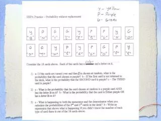
Jury Selection About 20% of adult residents in San Luis Obispo County (CA) are age 65 or older. a) If one adult is selected at random from this county, what is the probability that he/she will be age 65 or older? b) Suppose that a sample of 12 adults is randomly selected from this county, to form a jury. Guess the probability that at least one-third (4 or more people) of the jury are age 65 or older
Results of simulating 1000 such randomly selected juries. Observational unit: 1 jury of 12 people Variable measured: # senior citizens on the jury c) Use this histogram to approximate the probability that senior citizens (age 65 or older) would comprise at least 1/3 of the members of a randomly selected 12-person jury. How close to this probability was your guess in Question 2?
d) Now suppose that a sample of 75 adult residents is randomly selected from this county, perhaps to form a pool from which to choose a jury. Guess the probability that at least 1/3 of this pool of 75 people are age 65 or older. Results of simulating 1000 such randomly selected jury pools.
e) Use the histogram to approximate the probability that senior citizens would comprise at least 1/3 (i.e., 25 or more) of the members of a randomly selected 75-person jury pool. How close to this was your guess? f) For which sample size (12 or 15) is the sample (from a population containing 20% seniors) more likely to contain at least 1/3 seniors? Explain why this makes sense. g) For which sample size is the sample more likely to contain between 15% and 25% seniors seniors? Use the previous histograms to give a sensible answer.