Download

1 / 30
300 likes | 437 Views
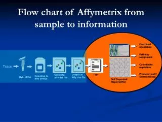
Flow chart of Affymetrix from sample to information. Functional annotation. Pathway assignment. Co-ordinate regulation. Tissue. Promoter motif commonalities. Output as Affy.chp file. Text. Generate Affy.dat file. Hybridize to Affy arrays. Hyb. cRNA. Self Organized Maps (SOMs).

E N D
Flow chart of Affymetrix from sample to information Functional annotation Pathway assignment Co-ordinate regulation Tissue Promoter motif commonalities Output as Affy.chp file Text Generate Affy.dat file Hybridize to Affy arrays Hyb. cRNA Self Organized Maps (SOMs)
Microarray Data Analysis • Data preprocessing and visualization • Supervised learning • Machine learning approaches • Unsupervised learning • Clustering and pattern detection • Gene regulatory regions predictions based co-regulated genes • Linkage between gene expression data and gene sequence/function databases • …
Data preprocessing • Data preparation or pre-processing • Normalization • Feature selection • Base on the quality of the signal intensity • Based on the fold change • T-test • …
Experiment1 Experiment2 Control Control Normalization • Need to scale the red sample so that the overall intensities for each chip are equivalent
Normalization • To insure the data are comparable, normalization attempts to correct the following variables: • Number of cells in the sample • Total RNA isolation efficiency • Signal measurement sensitivity • … • Can use simple math • Normalization by global scaling (bring each image to the same average brightness) • Normalization by sectors • Normalization to housekeeping genes • … • Active research area
Mn-SOD Annexin IV Aminoacylase 1 Basic Data Analysis • Fold change (relative change in intensity for each gene)
Microarray Data Analysis • Data preprocessing and visualization • Supervised learning • Machine learning approaches • Unsupervised learning • Clustering and pattern detection • Gene regulatory regions predictions based co-regulated genes • Linkage between gene expression data and gene sequence/function databases • …
Microarrays: An Example • Leukemia: Acute Lymphoblastic (ALL) vs Acute Myeloid (AML), Golub et al, Science, v.286, 1999 • 72 examples (38 train, 34 test), about 7,000 probes • well-studied (CAMDA-2000), good test example ALL AML Visually similar, but genetically very different
Probe AML1 AML2 AML3 ALL1 ALL2 ALL3 p-value D21869_s_at 170.7 55.0 43.7 5.5 807.9 1283.5 0.243 D25233cds_at 605 31.0 629.2 441.7 95.3 205.6 0.487 D25543_at 2148.7 2303.0 1915.5 49.2 96.3 89.8 0.0026 L03294_g_at 241.8 721.5 77.2 66.1 107.3 132.5 0.332 J03960_at 774.5 3439.8 614.3 556 14.4 12.9 0.260 M81855_at 1087 1283.7 1372.1 1469 4611.7 3211.8 0.178 L14936_at 212.6 2848.5 236.2 260.5 2650.9 2192.2 0.626 L19998_at 367 3.2 661.7 629.4 151 193.9 0.941 L19998_g_at 65.2 56.9 29.6 434.0 719.4 565.2 0.022 AB017912_at 1813.7 9520.6 2404.3 3853.1 6039.4 4245.7 0.963 AB017912_g_at 385.4 2396.8 363.7 419.3 6191.9 5617.6 0.236 U86635_g_at 83.3 470.9 52.3 3272.5 3379.6 5174.6 0.022 … … … … … … … … Feature selection
Hypothesis Testing • Null hypothesis is an hypothesis about a population parameter. • Hypothesis testing is to test the viability of the null hypothesis for a set of experimental data • Example: • Test whether the time to respond to a tone is affected by the consumption of alcohol • Hypothesis : µ1 - µ2 = 0 • µ1 is the mean time to respond after consuming alcohol • µ2 is the mean time to respond otherwise
Z-test • Theorem: If xi has a normal distribution with mean and standard deviation 2, i=1,…,n, then U= ai xi has a normal distribution with a mean E(U)= ai and standard deviation D(U)=2 ai 2. • xi /n ~ N(, 2/n). • Z test : H: µ = µ0 (µ0 and 0 are known, assume = 0) • What would one conclude about the null hypothesis that a sample of N = 46 with a mean of 104 could reasonably have been drawn from a population with the parameters of µ = 100 and = 8? Use Reject the null hypothesis.
Histogram Set 1 Set 2
Project 3 • A training data set • (38 samples, 7129 probes, 27 ALL, 11 AML) • A testing data set • (35 samples, 7129 probes, 22 ALL, 13 AML) • Lab today: pick the top probes that can differentiate the two sub types and process the testing data set
L L L M M M M M M M M M M M M L L L M M M L L L Feature 1 Feature 1 Feature 1 M M M L L L L L L L L L L L L Feature 2 Feature 2 Feature 2 = ALL = ALL L L = AML = AML M M = test sample = test sample K Nearest Neighbor Classification
Distance measures • Euclidean distance • Manhattan distance
test sample Feature0 Feature1 Feature50 … … M L M M Jury Decisions • Use one feature at a time for the classification • Combining the results from the top 51 features • Majority decision
False Discovery • Two possible errors in making a decision about the null hypothesis. • We could reject the null hypothesis when it is actually true, i.e., our results were obtained by chance. (Type I error). • We could fail to reject the null hypothesis when it is actually false, i.e. our experiment failed to detect the true difference that exists. (Type II error) • We set at a level which will minimize the chances of making either of these errors.
False Discovery • Type I error: False Discovery • False Discovery Rate (FDR) is equal to the p-value of the t-test X the number of genes in the array • For a p-value of 0.01 10,000 genes = 100 false “different” genes • You cannot eliminate false positives, but by choosing a more stringent p-value, you can keep them manageable (try p=0.001) • The FDR must be smaller than the number of real differences that you find - which in turn depends on the size of the differences and variability of the measured expression values
? RCC subtypes • Clear Cell RCC (70-80%) • Papillary (15-20%) • Chromoprobe (4-5%) • Collecting duct • Oncocytoma • Saramatoid RCC Goal: Identify a panel of discriminator genes
Genetic Algorithm for Feature Selection Raw measurement data Clear cell RCC, etc. Sample f1 f2 f3 f4 f5 Feature vector = pattern
Why Genetic Algorithm? • Assuming 2,000 relevant genes, 20 important discriminator genes (features). • Cost of an exhaustive search for the optimal set of features ? C(n,k)=n!/k!(n-k)! C(2,000, 20) = 2000!/(20!1980!) ≥ (100)^20 = 10^40 If it takes one femtosecond (10-15 second) to evaluate a set of features, it takes more than 310^17 years to find the optimal solution on the computer.
Evolutionary Methods • Based on the mechanics of Darwinian evolution • The evolution of a solution is loosely based on biological evolution • Population of competing candidate solutions • Chromosomes (a set of features) • Genetic operators (mutation, recombination, etc.) • generate new candidate solutions • Selection pressure directs the search • those that do well survive (selection) to form the basis for the next set of solutions.
A Simple Evolutionary Algorithm Increasing Fitness Evaluation Genetic Operators Selection
g100 g100 g2 g2 g5 g5 g7 g1 g2 g20 g21 g21 g3 g3 g6 g6 g7 g1 g2 g20 g10 g10 g22 g12 g15 g15 g7 g7 g12 g12 g1 g14 g21 g23 g51 g25 g7 g17 g20 g201 g10 g10 g23 g23 g56 g56 g72 g72 g25 g25 Genetic Algorithm Stop Good enough 4 3 2 Not good enough 1 5
Encoding • Most difficult, and important part of any GA • Encode so that illegal solutions are not possible • Encode to simplify the “evolutionary” processes, e.g. reduce the size of the search space • Most GA’s use a binary encoding of a solution, but other schemes are possible
GA Fitness • At the core of any optimization approach is the function that measures the quality of a solution or optimization. • Called: • Objective function • Fitness function • Error function • measure • etc.
Crossover Mutation 10 30 62 80 10 30 50 70 Randomly Selected Mutation Site 20 40 60 80 • Recombination is intended to produce promising individuals. • Mutation maintains population diversity, preventing premature convergence. Randomly Selected Crossover Point 10 30 60 80 20 40 50 70 Genetic Operators
Genetic Algorithm/K-Nearest Neighbor Algorithm Classifier (kNN) Feature Selection(GA) MicroarrayDatabase