Download
1 / 41
430 likes | 580 Views
Outline 1. Geochemistry of 14 C 2. Examples, with emphasis on scaling and testing models. For additional detail, see notes from Radiocarbon in Ecology and Earth System Science Short Course: https://webfiles.uci.edu/setrumbo/public/shortcourse/radiocarbon_short_course.html.

E N D
Outline • 1. Geochemistry of 14C • 2. Examples, with emphasis on scaling and testing models For additional detail, see notes from Radiocarbon in Ecology and Earth System Science Short Course: https://webfiles.uci.edu/setrumbo/public/shortcourse/radiocarbon_short_course.html
Radiocarbon is how we tell time in the carbon cycle The least abundant naturally occurring isotope of carbon: C-12 (98.8%) C-13 (1.1%) 14C (<10-10 %) or 1 14C : 1 trillion 12C 14C is the longest lived radioactive isotope of C, and decays to 14N by emitting a b particle (electron):
14C is continually produced in the upperatmosphere by nuclear reaction of nitrogen with cosmic radiation. Cosmic ray proton thermal neutron 14N nucleus 14C nucleus spallation products 14CO Oxidation, mixing Ocean/biosphere exchange stratosphere 14CO2 troposphere
Unlike stable isotopes, radiocarbon is constantly created and destroyed Loss by radioactive decay Production in stratosphere Total number of 14C atoms (N) in Earth’s C reservoirs -l N l = Radioactive decay constant, ~1/8267 years Total amount of radiocarbon on Earth can (and does) vary with factors that influence cosmic ray interaction with upper atmosphere
typical ratio of 14C/12C divided by the Modern (i.e. atmospheric) 14C/12C ratio Amount of carbon (x1016 moles) per cent of total 14C in the major global C reservoirs 6 1.01.7-2.0% Atmosphere (CO2) 30 0.958-10% 6 0.971.6-2% Surface Ocean (DIC) Terrestrial Biota 280 0.8465-78% 13 0.903-4% Deep Ocean (DIC) Soil Organic Matter 10 0.62% DOC Where the 14C is depends on (1) how much C is there (2) how fast it exchanges with the atmosphere 7-70 0.95 2-18% Coastal / Marine Sediment
Reporting of 14C data #1: Fraction Modern (FM) Corrected to a common d13C value (“Modern” is 1950) The 14C standard: Ninety-five percent of the activity of Oxalic Acid I
The 14C standard :Oxalic Acid I The principal modern radiocarbon standard is N.I.S.T Oxalic Acid I (C2H2O4), made from a crop of 1955 sugar beets. Ninety-five percent of the activity of Oxalic Acid I from the year 1950 is equal to the measured activity of the absolute radiocarbon standard which is 1890 wood (chosen to represent the pre-industrial atmosphere 14CO2), corrected for radioactive decay to 1950. This is Modern, or a 14C/12C ratio of 1.18x10⁻¹², which decays at a rate of 13.6 dpm per gram carbon.
Reporting of 14C data #2: Radiocarbon Age Radioactivity = number of decays per unit time = dN/dt dN/dt = -l14N, where N is the number of 14C atoms; dN/N = -l14dt T = (-1/ l14)ln (N(t)/N(0)) If radiocarbon production rate and its distribution among Atmosphere, ocean and terrestrial reservoirs is constant, Then N(0) = atmospheric 14CO2 value(i.e. Modern). F Drops to 0.5 in 5730 years (t1/2) Drops to 0.25 in 2*t1/2 years t1/2 Years
Radiocarbon Age (Libby age) Radiocarbon Age = -(1/l14)*ln(FM) Where FM is Fraction Modern andl14 is the decay constant for 14C The half life (t1/2 = ln(2)/l14) used to calculate radiocarbon ages is the one first used by Libby (5568 years). A more recent and accurate determination of the half-life is 5730 years. To convert a radiocarbon age to a calendar age, the tree ring calibration curve is used. Remember that the “age” reported by 14C labs uses an ‘incorrect’ half-life for geochemical purposes; that “age” is NOT a residence time!
The second way to make radiocarbon - “bomb 14C”- makes 14C a useful tracer of the global C cycle over the last 50 years
http://www.iup.uni-heidelberg.de/institut/forschung/groups/kk/14co2.htmlhttp://www.iup.uni-heidelberg.de/institut/forschung/groups/kk/14co2.html
For tracking bomb 14C we use yet another way of expressing 14C data: Deviation in parts per thousand (per mil, ‰) from the isotopic ratio of an absolute standard (like stable isotope notation) Corrects for decay of OX1 standard since 1950 This gives an absolute value of radiocarbon that does not change with time
Wait - We know 13C is fractionated by kinetic and equilibrium processes because of its mass – so 14C must be too!How does that affect ages, etc? Remember FM are corrected to a common 13C value and therefore 14C values reported as fraction Modern, Libby Age, or D14C do not reflect mass-dependent fractionation of isotopes. The sample is corrected to have d13C of -25 ‰ (14C is either added or subtracted, assuming 14C is fractionated twice as much as 13C)
Why must there be a correction for mass dependent fractionation? CO2 in air d13C = -8 ‰ Leaf d13C = -28 ‰ 14C-12C mass difference is ~twice that of 13C–12C Therefore a 20 ‰ difference in 13C means ~ 40 ‰ difference in 14C Expressed as an ‘age’ this is -8033*ln(.96) = 330 years Tocorrect using 14C/12C:
Examples of using radiocarbon for spatial extrapolation/model testing: • The “Suess” effect and isodisequilibrium • A direct test for ecosystem carbon cycle models (how many soil pools?) • Partitioning soil respiration sources
SUESS HERADIOCARBON CONCENTRATION IN MODERN WOOD, SCIENCE, 122 (3166): 415-417 1955 The Suess Effect Atmosphere - Carbon dioxide (gas) CO2 Methane (gas) CH4 Ocean - dissolved ions (bicarbonate and carbonate) + organic matter Land - Organic matter - Carbon is a constituent of all living things Land, air, water Fossil organic matter (coal, petroleum, natural gas) OLD, NO RADIOCARBON Limestone (solid) CaCO3 Solid Earth
Suess effect in 13C: Depletion of Atmospheric d13C by Fossil Fuels AND Deforestation (land C source to atmosphere) d13C (per mil) CO2 (ppm) Francey et al. [1999]
What makes us sure CO2 increase is caused by humans? Suess effect in radiocarbon - depletes 14C Tree rings Broecker et al. 1983
Because the atmosphere is changing with time in 13C and 14C, Isotopic reservoirs in ocean or land reservoirs that are not in steady state with the contemporary atmosphere; degree of ‘isodisequilibrium’ varies with size of gross exchange with atmosphere and mean age of respired CO2 Gba Gab Fung et al. 1997 GBC -6.5 Atm. d13C (‰) tb Isotopic Disequilibrium -8.0 time tb = Mean Residence Time
Example of a mass balance: What is the 14C signature of CO2 being respired from soil and accumulating in a chamber? 40 minutes 1000 ppm D14C = 95‰ 380 ppm D14C = 60‰ CO2 mass balance: 380 ppm + X = 1000 ppm X = 620 ppm 14C mass balance: 380ppm* 60‰ + 620ppm*Y‰ = 1000ppm*95‰ Y = 116‰
Radiocarbon of soil-respired CO2 provides a direct measure of isodisequilibrium “mean age” of several years up to a decade D14C D14C
Model Prediction of 14C in atmospheric CO2 in current boundary layer Lows in northern hemisphere from fossil fuel burning Max. at equator; biosphere recycling (large GPP and lag of several years) Krakauer et al. Tellus (in press) See also Randerson et al. 2002 GBC
Continental Variations in Atmospheric D14C measured using annual plants Δ14C measurements of corn from the continental U.S. during the summer of 2004 Hsueh et al Geophy. Res. Lett. (2007)
Tests many aspects of carbon cycle, tracer transport models: Boundary layer ventilation** Spatial distribution of fossil fuel sources** Mean of respired CO2 Hsueh et al. [GRL 2007] Annual plants are imperfect recorders (biased to am hours?, spring season)
Examples of using radiocarbon for spatial extrapolation/model testing: • The “Suess” effect and isodisequilibrium • A direct test for ecosystem carbon cycle models (how many soil pools?) • Partitioning soil respiration sources
Examples of using radiocarbon for spatial extrapolation/model testing: • The “Suess” effect and isodisequilibrium • A direct test for ecosystem carbon cycle models (how many soil pools?) • Partitioning soil respiration sources
Simplified soil C cycle CO2 Key factors: climate, vegetation mineralogy, time. Plant Litter Microbes Microbial Byproducts Stabilized SOM Carbon Pools in Models DOC Metabolic and Resistant Plant Material Microbial Active Passive Slow Days Years Decades Centuries Millennia Time
Approach 1. Attempt to match model pools to physically and chemically isolated fractions in soils Problem: We do not yet have fractionation methods that unequivocally isolate homogeneous fractions analogous to those in models Plant Litter Microbes Low density > Silt size Microbial Byproducts Stabilized SOM PLFA incubations Low density < Silt size High density Metabolic and Resistant Plant Material Microbial Active Passive Slow
Physical and chemical separation of soils can help isolate pools with different turnover timesHowever, even these pools contain both faster- and slower-cycling material Density separation Flotation, sieving Low density +100‰ Detritus +200‰ High density +50‰ Extraction with acids and bases Microbially altered material (humus) +90‰ Hydrolyzate Residue -180‰ Bulk soil +70 ‰
14C signature of terrestrial carbon pools atmosphere turnover time 1000 800 3 yr With only one data point, non-unique solution 600 14C (‰) 400 30 yr 200 80 yr 0 -200 1950 1960 1970 1980 1990 2000 Year Turnover time = 1/k C(t) * R(p) = I * R(atm) + C(t-1) * R(p-1)- k * C(t-1) * R(p-1) - * C(t-1) * R(p-1)
Approach 2. Use CO2 derived from microbial respiration as a direct measure of the time lag between fixation and decomposition CO2 Allows more direct comparison with ecosystem model predictions Plant Litter Microbes Microbial Byproducts Stabilized SOM Metabolic and Resistant Plant Material Microbial Active Slow Passive
Data from these field sites: Boreal forest, central Manitoba (NOBS) Temperate Mixed (Harvard) and conifer (Howland) forests Sierra Nevada Elevation gradient (temperature and vegetation change with elevation) Tropical Forest (Manaus, Santarem, Brazil) Heterotrophic Respiration is measured by putting litter and 0-10 cm soil cores in sealed jars, then measuring the rate of CO2 evolution and the isotopic signature of evolved CO2. Short-term incubations; large roots removed, all at 23 C and field moisture, except boreal soils (incubated at average in situ temperatures)
Data for O horizon (surface layer) Incubations for four forest types ~5 years D14C D14C Year
DD14C (D14CCO2 - D14Catm) of respired CO2 Measurements suggest strong temperature sensitivity Latitudinal gradient compared to Sierra Nevada Litter/O horizon Mineral Soil DD14C Site Mean Annual Temperature
DD14C (D14CCO2 - D14Catm) of respired CO2 Measurements suggest strong temperature sensitivity Latitudinal gradient compared to Sierra Nevada Litter/O horizon 0-5 cm Mineral Soil ~ 15 years DD14C ~15 years > 50 years ~3 years ~2-3 years Site Mean Annual Temperature
Estimate age of respired CO2 using a pulse-response experiment for CASA Tropical forest Temperate forest CO2 respired Boreal forest Thompson,and Randerson, Global Change Biol., 1999. Years since pulse
CASA pulse response function provides a prediction of the 14C of heterotrophically respired CO2 400 S Amount of C respired in year i Atmosphere D14C in year i X i=0 400 S Amount of C respired in year i i=0
Comparison to CASA Prediction: Example for the tropics Litter/O horizon Mineral Soil Control No Wood DD14C Site Mean Annual Temperature
Comparison to CASA Prediction – CASA has shorter lag at low temperature Longer lag at high temperature Litter/O horizon Mineral Soil Control No Wood DD14C Site Mean Annual Temperature
Comparison to CASA Prediction – Removing inputs from coarse wood debris improves agreement in the tropics Litter/O horizon Mineral Soil Control No Wood DD14C Site Mean Annual Temperature
Isotopes of C contain independent information • 13C = integrates multiple physiological processes • 14C = time since C assimilation; includes time in the plant! See Radiocarbon Short Course for more!