Download
1 / 26
280 likes | 508 Views
Random Effects Models for Panel Data. Peter W. F. Smith University of Southampton. Overview. Regression for longitudinal data Random intercept models Estimation Gender role attitudes example Random slope (coefficient) models. Regression for longitudinal data. For repeated measure data

E N D
Random Effects Models for Panel Data Peter W. F. Smith University of Southampton
Overview • Regression for longitudinal data • Random intercept models • Estimation • Gender role attitudes example • Random slope (coefficient) models
Regression for longitudinal data For repeated measure data yiji = 1,…, m j= 1,…, ni consider the model Example yij = gender role score for subject i,j = 1,…, 4 xij = years since 1991, i.e., xi1 = 0, xi2 = 2, xi3 = 4, xi4 = 6
Regression for longitudinal data (cont) If we can assume εij has mean zero and independent for different i or j, then we can use standard methods to fit the model Problem: Unlikely that εij is independent of εik for j≠k
Regression for longitudinal data (cont) If we include more covariates into the model: Thenεij may be more like ‘random shocks’ and independence assumption may be more plausible However, still likely to be unmeasured individual factors which lead to a positive correlation between εij and εik for j≠k
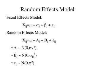
Random intercept models To address problem, consider alternative model where ui is the subject-specific residual and represents unmeasured individual factors which affect y
Random intercept models (cont) • Fixed effects model - assume the ui are fixed • Random effects model - assume the ui are random with • zero mean • Var(ui) = σu2 • Cor(ui, εij) = 0 If Var(εij) = σε2then Var(yij) = σu2 + σε2
Estimation • For standard regression models, we can use ordinary least squares (OLS) methods for estimation • However, random effects models require more sophisticated methods such as • maximum likelihood estimation (MLE) • generalised least square (GLS) • restricted maximum likelihood (REML) estimation
Gender role attitudes example First consider time as a factor: where the dummy variables xij2 = 1 if j = 2, i.e., the observation was taken in 1993 0 otherwise xij3 = 1 if j = 3, i.e., the observation was taken in 1995 0 otherwise xij4 = 1 if j = 4, i.e., the observation was taken in 1997 0 otherwise
Gender role attitudes example (cont) Random-effects ML regression Number of obs = 5716 Group variable (i): pid Number of groups = 1429 Random effects u_i ~ Gaussian Obs per group: min = 4 avg = 4.0 max = 4 LR chi2(3) = 84.48 Log likelihood = -14013.56 Prob > chi2 = 0.0000 ------------------------------------------------------------------------------ score | Coef. Std. Err. z P>|z| [95% Conf. Interval] -------------+---------------------------------------------------------------- _Iyear_93 | -.0720784 .0817051 -0.88 0.378 -.2322174 .0880606 _Iyear_95 | -.4219734 .0817051 -5.16 0.000 -.5821124 -.2618344 _Iyear_97 | -.6585024 .0817051 -8.06 0.000 -.8186414 -.4983635 _cons | 20.31351 .0935197 217.21 0.000 20.13021 20.4968 -------------+---------------------------------------------------------------- /sigma_u | 2.779951 .0602025 46.18 0.000 2.661956 2.897946 /sigma_e | 2.183996 .0235861 92.60 0.000 2.137768 2.230223 -------------+---------------------------------------------------------------- rho | .6183509 .0117675 .5950898 .6411922 ------------------------------------------------------------------------------ Likelihood-ratio test of sigma_u=0: chibar2(01)= 2630.32 Prob>=chibar2 = 0.000
Gender role attitudes example (cont) Score decreases with time so consider time as a continuous variable and no other covariates: where xij = years since 1991 Also try including time-squared in the model
Gender role attitudes example (cont) Random-effects ML regression Number of obs = 5716 Group variable (i): pid Number of groups = 1429 Random effects u_i ~ Gaussian Obs per group: min = 4 avg = 4.0 max = 4 LR chi2(1) = 80.17 Log likelihood = -14015.718 Prob > chi2 = 0.0000 ------------------------------------------------------------------------------ score | Coef. Std. Err. z P>|z| [95% Conf. Interval] -------------+---------------------------------------------------------------- time | -.1162701 .0129252 -9.00 0.000 -.1416031 -.0909371 _cons | 20.37418 .0880119 231.49 0.000 20.20168 20.54668 -------------+---------------------------------------------------------------- /sigma_u | 2.779735 .0602076 46.17 0.000 2.66173 2.89774 /sigma_e | 2.185095 .0235981 92.60 0.000 2.138844 2.231347 -------------+---------------------------------------------------------------- rho | .6180766 .0117726 .594806 .6409282 ------------------------------------------------------------------------------ Likelihood-ratio test of sigma_u=0: chibar2(01)= 2627.65 Prob>=chibar2 = 0.000
Gender role attitudes example (cont) Random-effects ML regression Number of obs = 5716 Group variable (i): pid Number of groups = 1429 Random effects u_i ~ Gaussian Obs per group: min = 4 avg = 4.0 max = 4 LR chi2(2) = 82.19 Log likelihood = -14014.706 Prob > chi2 = 0.0000 ------------------------------------------------------------------------------ score | Coef. Std. Err. z P>|z| [95% Conf. Interval] -------------+---------------------------------------------------------------- time | -.0546011 .0452276 -1.21 0.227 -.1432456 .0340434 timesq | -.0102782 .0072237 -1.42 0.155 -.0244364 .0038801 _cons | 20.33307 .0926299 219.51 0.000 20.15151 20.51462 -------------+---------------------------------------------------------------- /sigma_u | 2.779836 .0602052 46.17 0.000 2.661836 2.897836 /sigma_e | 2.184579 .0235925 92.60 0.000 2.138339 2.23082 -------------+---------------------------------------------------------------- rho | .6182053 .0117702 .5949391 .641052 ------------------------------------------------------------------------------ Likelihood-ratio test of sigma_u=0: chibar2(01)= 2628.90 Prob>=chibar2 = 0.000
Gender role attitudes example (cont) Since timesq is not significant we remove it and add the other covariates: • Age • Sex • Educational attainment • Whether mother worked when subject was age 14 • Economic activity at time t (time varying)
Gender role attitudes example (cont) LR chi2(10) = 336.90 Log likelihood = -13887.349 Prob > chi2 = 0.0000 ------------------------------------------------------------------------------ score | Coef. Std. Err. z P>|z| [95% Conf. Interval] -------------+---------------------------------------------------------------- asex | 1.254086 .1510664 8.30 0.000 .9580015 1.550171 _Iaagecat_2 | -.5794384 .1831823 -3.16 0.002 -.938469 -.2204077 _Iaagecat_3 | -.7363652 .2092183 -3.52 0.000 -1.146425 -.3263049 _Iaagecat_4 | -1.653055 .2919503 -5.66 0.000 -2.225267 -1.080843 aeduc | .5435919 .152435 3.57 0.000 .2448248 .8423591 amumwk | 1.045323 .1544268 6.77 0.000 .7426517 1.347994 _Iecact_2 | -.516662 .1518656 -3.40 0.001 -.8143131 -.2190108 _Iecact_3 | -.3032344 .1082726 -2.80 0.005 -.5154448 -.0910241 _Iecact_4 | -1.88322 .1925009 -9.78 0.000 -2.260515 -1.505925 time | -.101087 .0131434 -7.69 0.000 -.1268476 -.0753264 _cons | 18.23961 .2891569 63.08 0.000 17.67288 18.80635 -------------+---------------------------------------------------------------- /sigma_u | 2.566197 .0569278 45.08 0.000 2.45462 2.677773 /sigma_e | 2.170336 .0234529 92.54 0.000 2.124369 2.216303 -------------+---------------------------------------------------------------- rho | .5829964 .0124132 .5585233 .6071519 ------------------------------------------------------------------------------ Likelihood-ratio test of sigma_u=0: chibar2(01)= 2282.21 Prob>=chibar2 = 0.000
Gender role attitudes example (cont) • All covariates are significant • Higher scores, on average, across the waves if: • younger • woman • more educated • mother worked • full-time worker • Lower scores if family carer • To assess changes with time interact covariates with time
Gender role attitudes example (cont) LR chi2(19) = 368.25 Log likelihood = -13871.676 Prob > chi2 = 0.0000 ------------------------------------------------------------------------------ score | Coef. Std. Err. z P>|z| [95% Conf. Interval] -------------+---------------------------------------------------------------- _Iasex_2 | 1.482231 .1698729 8.73 0.000 1.149287 1.815176 time | .0296569 .0358778 0.83 0.408 -.0406622 .0999761 _IaseXtime_2 | -.0771893 .0271185 -2.85 0.004 -.1303406 -.024038 _Iaagecat_2 | -.6598482 .2109859 -3.13 0.002 -1.073373 -.2463234 _Iaagecat_3 | -.7070063 .2405735 -2.94 0.003 -1.178522 -.2354909 _Iaagecat_4 | -1.524458 .3318926 -4.59 0.000 -2.174956 -.8739606 _IaagXtime_2 | .0303784 .0329981 0.92 0.357 -.0342968 .0950535 _IaagXtime_3 | -.0079801 .0374844 -0.21 0.831 -.0814481 .0654879 _IaagXtime_4 | -.0397846 .0515105 -0.77 0.440 -.1407434 .0611742 _Iaeduc_1 | .7771973 .1718789 4.52 0.000 .4403208 1.114074 _IaedXtime_1 | -.0767993 .0265393 -2.89 0.004 -.1288155 -.0247832 _Iamumwk_1 | 1.297623 .1740909 7.45 0.000 .9564114 1.638835 _IamuXtime_1 | -.0841219 .026807 -3.14 0.002 -.1366626 -.0315812
Gender role attitudes example (cont) _Iecact_2 | -.202959 .259161 -0.78 0.434 -.7109053 .3049873 _Iecact_3 | -.2475432 .1529072 -1.62 0.105 -.5472359 .0521494 _Iecact_4 | -1.432423 .4011378 -3.57 0.000 -2.218639 -.6462076 _IecaXtime_2 | -.0765033 .0612526 -1.25 0.212 -.1965563 .0435496 _IecaXtime_3 | -.0113124 .041113 -0.28 0.783 -.0918924 .0692676 _IecaXtime_4 | -.0984208 .085874 -1.15 0.252 -.2667307 .0698892 _cons | 19.08584 .2249966 84.83 0.000 18.64485 19.52682 -------------+---------------------------------------------------------------- /sigma_u | 2.567637 .0569042 45.12 0.000 2.456107 2.679167 /sigma_e | 2.162468 .023372 92.52 0.000 2.11666 2.208277 -------------+---------------------------------------------------------------- rho | .5850335 .0123854 .5606114 .6091312 ------------------------------------------------------------------------------ Likelihood-ratio test of sigma_u=0: chibar2(01)= 2296.07 Prob>=chibar2 = 0.000 p-values for coefficients for interactions of time with age and economic activity suggest these are non-significant and a likelihood-ratio test confirms this, so remove them
Gender role attitudes example (cont) Log likelihood = -13874.394 Prob > chi2 = 0.0000 ------------------------------------------------------------------------------ score | Coef. Std. Err. z P>|z| [95% Conf. Interval] -------------+---------------------------------------------------------------- _Iasex_2 | 1.488305 .168601 8.83 0.000 1.157853 1.818756 time | .0203711 .0274851 0.74 0.459 -.0334986 .0742408 _IaseXtime_2 | -.0814268 .0260717 -3.12 0.002 -.1325265 -.0303272 _Iaagecat_2 | -.5790363 .1832745 -3.16 0.002 -.9382478 -.2198248 _Iaagecat_3 | -.7360443 .2093247 -3.52 0.000 -1.146313 -.3257754 _Iaagecat_4 | -1.652975 .2921061 -5.66 0.000 -2.225492 -1.080457 _Iaeduc_1 | .7548028 .1708656 4.42 0.000 .4199124 1.089693 _IaedXtime_1 | -.0696087 .0256519 -2.71 0.007 -.1198856 -.0193318 _Iamumwk_1 | 1.279404 .1736561 7.37 0.000 .9390445 1.619764 _IamuXtime_1 | -.0779366 .0264326 -2.95 0.003 -.1297434 -.0261297 _Iecact_2 | -.4512691 .1523927 -2.96 0.003 -.7499533 -.1525848 _Iecact_3 | -.2887654 .1081209 -2.67 0.008 -.5006785 -.0768523 _Iecact_4 | -1.807042 .1944702 -9.29 0.000 -2.188197 -1.425888 _cons | 19.12255 .2099684 91.07 0.000 18.71102 19.53408 -------------+---------------------------------------------------------------- /sigma_u | 2.569273 .0569294 45.13 0.000 2.457694 2.680853 /sigma_e | 2.163402 .0233812 92.53 0.000 2.117576 2.209229 -------------+---------------------------------------------------------------- rho | .5851332 .0123818 .560718 .6092239 ------------------------------------------------------------------------------ Likelihood-ratio test of sigma_u=0: chibar2(01)= 2298.93 Prob>=chibar2 = 0.000
Gender role attitudes example (cont) Conclusions • Initially, higher scores if: • younger • woman • more educated • mother worked • full-time worker • Scores decrease, compared to baseline men’s scores, if: • woman • more educated • mother worked
Gender role attitudes example (cont) • Between, σu2, and within, σe2, subject variation similar • Intra-class correlation or within-subject correlation: • estimated to be 0.59 • proportion of total variation between subjects • exchangeable structure imposed
Random slope (coefficient) models • We can allow the coefficients to be random: where βi is a vector of subject-specific random coefficients with mean β uiis a subject-specific random intercept with mean zero bi is a subject-specific random deviation from mean coefficient • No longer imposes exchangeable correlation structure
Random slope (coefficient) models (cont) Example: random slope model where yij = gender role score for subject i,j = 1,…, 4 xij = years since 1991, i.e., xi1 = 0, xi2 = 2, xi3 = 4, xi4 = 6 β1 = mean slope bi = subject-specific random deviation from mean slope ui = subject-specific random intercept
Gender role attitudes example (cont) Mixed-effects ML regression Number of obs = 5716 Group variable: pid Number of groups = 1429 Obs per group: min = 4 avg = 4.0 max = 4 Wald chi2(1) = 61.81 Log likelihood = -13968.202 Prob > chi2 = 0.0000 ------------------------------------------------------------------------------ score | Coef. Std. Err. z P>|z| [95% Conf. Interval] -------------+---------------------------------------------------------------- time | -.1162701 .0147891 -7.86 0.000 -.1452562 -.087284 _cons | 20.37418 .0903998 225.38 0.000 20.197 20.55136 ------------------------------------------------------------------------------ ------------------------------------------------------------------------------ Random-effects Parameters | Estimate Std. Err. [95% Conf. Interval] -----------------------------+------------------------------------------------ pid: Unstructured | sd(time) | .3327505 .0193146 .2969685 .3728439 sd(_cons) | 2.975303 .0744852 2.832839 3.124933 corr(time,_cons) | -.326163 .0438536 -.4092518 -.2377091 -----------------------------+------------------------------------------------ sd(Residual) | 2.009102 .0265739 1.957687 2.061867 ------------------------------------------------------------------------------ LR test vs. linear regression: chi2(3) = 2722.68 Prob > chi2 = 0.0000 Note: LR test is conservative and provided only for reference
Gender role attitudes example (cont) Log likelihood = -13836.328 Prob > chi2 = 0.0000 ------------------------------------------------------------------------------ score | Coef. Std. Err. z P>|z| [95% Conf. Interval] -------------+---------------------------------------------------------------- _Iasex_2 | 1.48562 .1719744 8.64 0.000 1.148556 1.822684 time | .0203335 .0310106 0.66 0.512 -.0404462 .0811131 _IaseXtime_2 | -.0840355 .0293473 -2.86 0.004 -.1415552 -.0265158 _Iaagecat_2 | -.582097 .1834402 -3.17 0.002 -.9416331 -.2225609 _Iaagecat_3 | -.7345624 .2095101 -3.51 0.000 -1.145195 -.3239303 _Iaagecat_4 | -1.64792 .2922832 -5.64 0.000 -2.220785 -1.075056 _Iaeduc_1 | .7579772 .1741799 4.35 0.000 .4165909 1.099363 _IaedXtime_1 | -.0694669 .0289575 -2.40 0.016 -.1262226 -.0127111 _Iamumwk_1 | 1.279735 .1771255 7.23 0.000 .9325754 1.626895 _IamuXtime_1 | -.0776092 .0298465 -2.60 0.009 -.1361072 -.0191113 _Iecact_2 | -.4208602 .1525266 -2.76 0.006 -.719807 -.1219135 _Iecact_3 | -.2720734 .1089196 -2.50 0.012 -.4855519 -.058595 _Iecact_4 | -1.691365 .1946089 -8.69 0.000 -2.072791 -1.309938 _cons | 19.1156 .2132541 89.64 0.000 18.69763 19.53357 ------------------------------------------------------------------------------
Gender role attitudes example (cont) ------------------------------------------------------------------------------ Random-effects Parameters | Estimate Std. Err. [95% Conf. Interval] -----------------------------+------------------------------------------------ pid: Unstructured | sd(time) | .3109998 .0199229 .2743035 .3526052 sd(_cons) | 2.731567 .0718112 2.594384 2.876003 corr(time,_cons) | -.3057609 .0478012 -.3962674 -.2093691 -----------------------------+------------------------------------------------ sd(Residual) | 2.008425 .0266227 1.956917 2.061288 ------------------------------------------------------------------------------ LR test vs. linear regression: chi2(3) = 2375.06 Prob > chi2 = 0.0000 Note: LR test is conservative and provided only for reference