Download
1 / 38
430 likes | 1.28k Views
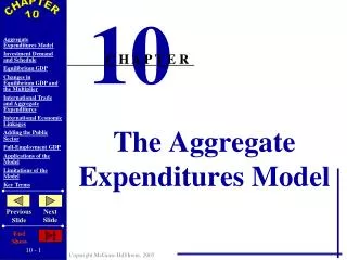
10. C H A P T E R. The Aggregate Expenditures Model. Simplifying Assumptions for the Private Closed-Economy model. Assumptions: A c losed economy with no international trade (no exports or imports). Government is ignored (no government purchases and no taxes).

E N D
10 C H A P T E R The Aggregate Expenditures Model
Simplifying Assumptions for the Private Closed-Economy model Assumptions: • A closed economy with no international trade (no exports or imports). • Government is ignored (no government purchases and no taxes). • Although both households and businesses save, we assume here that all saving is personal. • Depreciation and net foreign income are assumed to be zero for simplicity. • The economy has excess production capacity, so an increase in AD will raise output and employment, but not prices.
Two reminders concerning the assumptions: • They leave out two key components of aggregate demand (government spending and foreign trade), because they are largely affected by influences outside the domestic market system. 2. With no government or foreign trade, GDP, national income (NI), personal income (PI), and disposable income (DI) are all the same.
Tools of Aggregate Expenditures Theory: Consumption and Investment Schedules • The theory assumes that the level of output and employment depend directly on the level of aggregate expenditures. Changes in output reflect changes in aggregate spending. • In a closed private economy the two components of aggregate expenditures are: • Consumption (C). • Gross investment (Ig).
Investment Schedule: • The relationship between investment and GDPshows the amounts business firms collectively intend to invest at each possible level ofGDP or DI. • In developing the investment schedule, it is assumed that investment is independent of the current income. • The assumption that investment is independent of income is a simplification, but it will be used here.
Model Simplifications • Investment demand vs. schedule Investment Demand Curve Investment Schedule Investment Demand Curve Investment Schedule Ig 20 Investment (billions of dollars) r and i (percent) 8 20 20 ID 20 Real GDP (billions of dollars) Investment (billions of dollars)
Equilibrium GDP: Expenditures-Output Approach • Recall that consumption level is directly related to the level of income and that here income is equal to output level. • Investment is independent of income here and is planned or intended regardless of the current income situation. • Equilibrium GDP is the level of output whose production will create total spending just sufficient to purchase that output. Otherwise there will be a disequilibrium situation.
Equilibrium GDP (2) Real Domestic Output (and Income) (GDP=DI) (3) Con- sump- tion (C) (7) Unplanned Changes in Inventories (+ or -) (8) Tendency of Employment, Output, and Income (5) Investment (Ig) (6) Aggregate Expenditures (C+Ig) (1) Employ- ment (4) Saving (S) (1) – (2) …in Billions of Dollars In millions • 40 • 45 • 50 • 55 • 60 • 65 • 70 • 75 • 80 • 85 $370 390 410 430 450 470 490 510 530 550 $375 390 405 420 435 450 465 480 495 510 $-5 0 5 10 15 20 25 30 35 40 20 20 20 20 20 20 20 20 20 20 $395 410 425 440 455 470 485 500 515 530 Increase Increase Increase Increase Increase Equilibrium Decrease Decrease Decrease Decrease $-25 -20 -15 -10 -5 0 +5 +10 +15 +20
At levels below equilibrium, businesses will adjust to excess demand (revealed by the declining inventories) by stepping up production. They will expand production at any level of GDP less than the $470 billion equilibrium. As GDP rises, the number of jobs and total income will also rise • At levels of GDP above equilibrium, aggregate expenditures will be less than GDP. Businesses will have unsold output (Unplanned inventory investment) and will cut back on the rate of production. As GDP declines, the number of jobs and total income will also decline, but eventually the GDP and aggregate spending will be in equilibrium at $470 billion.
o 45 EQUILIBRIUM GDP (C + Ig = GDP) C + Ig $530 510 490 470 450 430 410 390 370 Equilibrium C Ig = $20 Billion Private spending, C + I g (billions of dollars) C =$450 Billion o 370 390 410 430 450 470 490 510 530 550 Real domestic product, GDP (billions of dollars)
EQUILIBRIUM GDP • At equilibrium, saving (leakage) and Planned Investment (injection) are Equal: • Leakage = Injection • (S) = (I) • or • No Unplanned Changes in Inventories (Unplanned inventory = 0) • Disequilibrium • Above Equilibrium • Leakage (S) > Injection (I) • Unplanned inventory accumulation
Below Equilibrium • Leakage (S) < Injection (I) • Unplanned inventory depletion • Saving represents a “leakage” from spending stream and causes (C) to be less than GDP. • Some of output is planned for business investment and not consumption, so this investment spending can replace the leakage due to saving.
Unplanned expenditures The unplanned portion is reflected as a business expenditure, even though the business may not have desired it, because the total output has a value that belongs to someone - either as a planned purchase or as an unplanned inventory. • If aggregate spending is less than equilibrium GDP, then businesses will find themselves with unplanned inventory investment on top of what was already planned. • If aggregate expenditures exceed GDP, then there will be less inventory investment than businesses planned as businesses sell more than they expected. This is reflected as a negative amount of unplanned investment in inventory. • At equilibrium there are no unplanned changes in inventory.
Quick Review • Equilibrium GDP is where aggregate expenditures equal real domestic output: C + planned Ig = GDP • A difference between saving and planned investment causes a difference between the production and spending plans of the economy as a whole. • A difference between production and spending plans leads to unintended inventory investment or unintended decline in inventories. • As long as unplanned changes in inventories occur, businesses will revise their production plans upward or downward until the investment in inventory is equal to what they planned. • Only where planned investment and saving are equal there will be no unintended investment or disinvestment in inventories to drive the GDP down or up.
Changes in Equilibrium GDP and the Multiplier • An initial change in spending (caused by shifts in C and I) will be acted on by the multiplier to produce larger changes in output. • The “initial change” is in planned investment spending. It could also result from a non-income-induced changes in consumption. Impact of changes in investment. Suppose investment spending rises by 5 billion (due to a rise in expected rate of return or to a decline in interest rates). • The increase in aggregate expenditures from investment leads to an increase in equilibrium GDP (size depends on the multiplier). 2. Conversely, a decline in investment spending leads to a decrease in equilibrium GDP (size depends on the multiplier).
CHANGES IN EQUILIBRIUM GDP AND THE MULTIPLIER Equilibrium GDP at Ig1level of investment Equilibrium GDP at Ig0level of investment o 45 510 490 470 450 430 (C + Ig ) 1 (C + Ig ) 0 Increases in the level of C + Ig Private spending (billions of dollars) o 430 450 470 490 510 Real domestic product, GDP (billions of dollars)
CHANGES IN EQUILIBRIUM GDP AND THE MULTIPLIER o 45 Equilibrium GDP at Ig2level of investment 510 490 470 450 430 (C + Ig ) 0 (C + Ig ) 2 Private spending (billions of dollars) Decreases in the level of C + Ig o 430 450 470 490 510 Real domestic product, GDP (billions of dollars)
International Trade and Equilibrium Output • Net exports affect aggregate expenditures in an open economy. Exports expand aggregate spending and imports contract aggregate spending on domestic output. • Exports (X) create domestic production, income, and employment due to foreign spending on domestically produced goods and services. • Imports (M) reduce the sum of consumption and investment expenditures by the amount expended on imported goods, so this figure must be subtracted so as not to overstate aggregate expenditures on domestically produced goods and services.
The net export schedule • Shows hypothetical amount of net exports that will occur at each level of GDP. Note that we assume that net exports areindependent of the current GDP level. • Positive net exports increase aggregate expenditures beyond what they would be in a closed economy and thus have an expansionary effect. The multiplier effect also is at work. • Negative net exports decrease aggregate expenditures beyond what they would be in a closed economy and thus have a contractionary effect. The multiplier effect also is at work here.
510 490 470 450 430 Aggregate Expenditures (billions of dollars) 45° 430 450 470 490 510 Real GDP (billions of dollars) +5 0 -5 Net Exports Xn (billions of Dollars) Real GDP Net Exports and Equilibrium GDP C + Ig+Xn1 C + Ig Aggregate Expenditures with Positive Net Exports C + Ig+Xn2 Aggregate Expenditures with Negative Net Exports Positive Net Exports Xn1 450 470 490 Xn2 Negative Net Exports
International economic linkages • Prosperity abroad: generally raises our exports and transfers some of their prosperity to us. (Conversely, recession abroad has the reverse effect.) • Tariffs on Kuwaiti products: may reduce our exports and depress our economy, causing us to retaliate and worsen the situation. • Changes in exchange rates: • Depreciation of the KD lowers the cost of Kuwaiti goods to foreigners and encourages exports from Kuwait, while discouraging the purchase of imports in Kuwait. This could lead to higher real GDP or to inflation, depending on the domestic employment situation. • Appreciation of the KD could have the opposite impact.
-700 200 150 100 50 0 50 100 150 200 250 Net Exports of Goods Select Nations, 2006 Negative Net Exports Positive Net Exports +31 Canada France -45 Japan +70 Italy -27 +203 Germany United Kingdom -171 -881 United States Source: World Trade Organization
Adding the Public Sector Simplifying assumptions: • Simplified investment and net export schedules are used. Assume they are independent of the level of current GDP. • Assume government purchases do not impact private spending schedules. • Assume that net tax revenues are derived entirely from personal taxes so that GDP, NI, and PI remain equal. • Assume that tax collections are independent of GDP level (i.e., it is a lump-sum tax) 5. The price level is assumed to be constant unless otherwise indicated.
Impact of government spending • Increases in government spending boost aggregate expenditures. It is subject to the multiplier effect. Impact of Taxes • Taxes reduce DI and, therefore, consumption and saving at each level of GDP. • An increase in taxes will lower the aggregate expenditures schedule relative to the 45-degree line and reduce the equilibrium GDP, and a decrease in tax will do the opposite. • At equilibrium GDP, the sum of leakages equals the sum of injections, i.e., Saving + Imports + Taxes = Investment + Exports + Government Purchases. (leakage) = (injection)
(1) Level of Output and Income (GDP=DI) (5) Net Exports (Xn) (7) Aggregate Expenditures (C+Ig+Xn+G) (2)+(4)+(5)+(6) (2) Consump- tion (C) (4) Investment (Ig) (6) Government (G) Exports (X) Imports (M) (3) Saving (S) Adding the Public Sector …in Billions of Dollars • $370 • 390 • 410 • 430 • 450 • 470 • 490 • 510 • 530 • 550 $375 390 405 420 435 450 465 480 495 510 $-5 0 5 10 15 20 25 30 35 40 $20 20 20 20 20 20 20 20 20 20 10 10 10 10 10 10 10 10 10 10 10 10 10 10 10 10 10 10 10 10 20 20 20 20 20 20 20 20 20 20 $415 430 445 460 475 490 505 520 535 550
ADDING THE PUBLIC SECTOR o 45 Government Purchases and Equilibrium GDP C + Ig + Xn + G Government Spending of $20 Billion C + Ig + Xn C Aggregate Expenditures (billions of dollars) o 470 550 Real domestic product, GDP (billions of dollars)
o 45 ADDING THE PUBLIC SECTOR Lump-Sum Tax and Equilibrium GDP $15 Billion Decrease in Consumption from a $20 Billion Increase in Taxes C + Ig + Xn + G Ca + Ig + Xn + G Aggregate Expenditures (billions of dollars) o 490 550 Real domestic product, GDP (billions of dollars)
Government purchases and taxes have different impacts. • Equal additions in government spending and taxation increase the equilibrium GDP. • If G and T are each increased by a particular amount, the equilibrium level of real output will rise by that same amount. b. Example, an increase of $20 billion in G and an offsetting increase of $20 billion in T will increase equilibrium GDP by $20 billion.
Explanation • An increase in G is direct and adds $20 billion to aggregate expenditures. • An increase in T has an indirect effect on aggregate expenditures because T reduces disposable incomes first, and then C falls by the amount of the tax times MPC. • The overall result is a rise in initial spending of $20 billion minus a fall in initial spending of $15 billion (.75 x $20 billion), which is a net upward shift in aggregate expenditures of $5 billion. • When this is subject to the multiplier effect, which is 4 (MPC =.75) in this example, the increase in GDP will be equal to $4 × $5 billion or $20 billion, which is the size of the change in G.
Injections, Leakages, and Unplanned Changes in Inventories – Equilibrium revisited • As demonstrated earlier, in a closed private economy equilibrium occurs when saving (a leakage) equals planned investment (an injection). • With the introduction of a foreign sector (net exports) and a public sector (government), new leakages and injections are introduced. 1. Imports and taxes are added leakages. 2. Exports and government purchases are added injections.
Equilibrium is found when the leakages equal the injections. When leakages equal injections, there are no unplanned changes in inventories. Symbolically, equilibrium occurs when: Sa + M + T = Ig + X + G where Sa is after-tax saving, M is imports, T is taxes, Ig is (gross) planned investment, X is exports, and G is government purchases.
Equilibrium vs. Full-Employment GDP • A recessionary expenditure gap exists when equilibrium GDP is below full-employment GDP. • A recessionary gap is the amount by which aggregate expenditures fall short of those required to achieve the full-employment level of GDP, or the amount by which the schedule would have to shift upward to realize the full-employment GDP. • The effect of the recessionary gap is to pull down the prices of the economy’s output.
An inflationary gap exists when aggregate expenditures exceed full-employment GDP, it exists when aggregate spending exceeds what is necessary to achieve full employment. • The inflationary gap is the amount by which the aggregate expenditures schedule must shift downward to realize the full-employment noninflationary GDP. • The effect of the inflationary gap is to pull up the prices of the economy’s output.
o 45 FULL-EMPLOYMENT GDP Recessionary Gap AE0 530 510 490 AE1 Recessionary Gap = $5 Billion Aggregate Expenditures (billions of dollars) Full Employment o 490 510 530 Real domestic product, GDP (billions of dollars)
o 45 FULL-EMPLOYMENT GDP Inflationary Gap AE2 Inflationary Gap = $5 Billion AE0 530 510 490 Aggregate Expenditures (billions of dollars) Full Employment o 490 510 530 Real domestic product, GDP (billions of dollars)
Last Word: Say’s Law, The Great Depression, and Keynes • Until the Great Depression of the 1930, most economists going back to Adam Smith had believed that a market system would ensure full employment of the economy’s resources except for temporary, short-term upheavals. • If there were deviations, they would be self-correcting. A slump in output and employment would reduce prices, which would increase consumer spending; would lower wages, which would increase employment again; and would lower interest rates, which would expand investment spending.
Say’s law, attributed to the French economist J. B. Say in the early 1800s, summarized the view in a few words: “Supply creates its own demand.” • Say’s law is easiest to understand in terms of barter. The woodworker produces furniture in order to trade for other needed products and services. All the products would be traded for something, or else there would be no need to make them. Thus, supply creates its own demand. • The Great Depression of the 1930s was worldwide. GDP fell by 40 percent in U.S. and the unemployment rate rose to nearly 25 percent. The Depression seemed to refute the classical idea that markets were self-correcting and would provide full employment.
John Maynard Keynes in 1936 in his General Theory of Employment, Interest, and Money, provided an alternative to classical theory, which helped explain periods of recession. • Not all income is always spent, contrary to Say’s law. • Producers may respond to unsold inventories by reducing output rather than cutting prices. • A recession or depression could follow this decline in employment and incomes.