Machine Learning – Lecture 4

1. Machine Learning – Lecture 4 Linear Discriminant Functions 19.04.2012 Bastian Leibe RWTH Aachen http://www.mmp.rwth-aachen.de leibe@umic.rwth-aachen.de Many slides adapted from B. Schiele TexPoint fonts used in EMF. Read the TexPoint manual before you delete this box.: AAAAAAAAAAAAAAAAAAAAAAAAAAAA

2. Course Outline • Fundamentals (2 weeks) • Bayes Decision Theory • Probability Density Estimation • Discriminative Approaches (5 weeks) • Linear Discriminant Functions • Support Vector Machines • Ensemble Methods & Boosting • Randomized Trees, Forests & Ferns • Generative Models (4 weeks) • Bayesian Networks • Markov Random Fields B. Leibe

3. Recap: Mixture of Gaussians (MoG) • “Generative model” “Weight” of mixturecomponent 1 3 2 Mixturecomponent Mixture density B. Leibe Slide credit: Bernt Schiele

4. Recap: Estimating MoGs – Iterative Strategy • Assuming we knew the values of the hidden variable… ML for Gaussian #1 ML for Gaussian #2 assumed known 1 111 22 2 2 j • 1 111 00 0 0 • 0 000 11 1 1 B. Leibe Slide credit: Bernt Schiele

5. Recap: Estimating MoGs – Iterative Strategy • Assuming we knew the mixture components… • Bayes decision rule: Decide j = 1 if assumed known 1 111 22 2 2 j B. Leibe Slide credit: Bernt Schiele

6. Recap: K-Means Clustering • Iterative procedure • Initialization: pick K arbitrarycentroids (cluster means) • Assign each sample to the closestcentroid. • Adjust the centroids to be themeans of the samples assignedto them. • Go to step 2 (until no change) • Algorithm is guaranteed toconverge after finite #iterations. • Local optimum • Final result depends on initialization. B. Leibe Slide credit: Bernt Schiele

7. Recap: EM Algorithm • Expectation-Maximization (EM) Algorithm • E-Step: softly assign samples to mixture components • M-Step: re-estimate the parameters (separately for each mixture component) based on the soft assignments = soft number of samples labeled j B. Leibe Slide adapted from Bernt Schiele

8. Summary: Gaussian Mixture Models • Properties • Very general, can represent any (continuous) distribution. • Once trained, very fast to evaluate. • Can be updated online. • Problems / Caveats • Some numerical issues in the implementation  Need to apply regularization in order to avoid singularities. • EM for MoG is computationally expensive • Especially for high-dimensional problems! • More computational overhead and slower convergence than k-Means • Results very sensitive to initialization  Run k-Means for some iterations as initialization! • Need to select the number of mixture components K.  Model selection problem (see Lecture 10) B. Leibe

9. EM – Technical Advice • When implementing EM, we need to take care to avoid singularities in the estimation! • Mixture components may collapse onsingle data points.  Need to introduce regularization • Enforce minimum width for the Gaussians • E.g., by enforcing that none of its eigenvalues gets too small. • if ¸i < ² then ¸i = ² B. Leibe Image source: C.M. Bishop, 2006

10. Applications • Mixture models are used in many practical applications. • Wherever distributions with complexor unknown shapes need to berepresented… • Popular application in Computer Vision • Model distributions of pixel colors. • Each pixel is one data point in e.g. RGB space.  Learn a MoG to represent the class-conditional densities.  Use the learned models to classify other pixels. B. Leibe Image source: C.M. Bishop, 2006

11. Application: Color-Based Skin Detection • Collect training samplesfor skin/non-skin pixels. • Estimate MoG torepresent the skin/ non-skin densities skin Classify skin color pixels in novel images non-skin M. Jones and J. Rehg, Statistical Color Models with Application to Skin Detection, IJCV 2002.

12. Interested to Try It? • Here’s how you can access a webcam in Matlab: function out = webcam % uses "Image Acquisition Toolbox„ adaptorName = 'winvideo'; vidFormat = 'I420_320x240'; vidObj1= videoinput(adaptorName, 1, vidFormat); set(vidObj1, 'ReturnedColorSpace', 'rgb'); set(vidObj1, 'FramesPerTrigger', 1); out = vidObj1 ; cam = webcam(); img=getsnapshot(cam); B. Leibe

13. Topics of This Lecture • Linear discriminant functions • Definition • Extension to multiple classes • Least-squares classification • Derivation • Shortcomings • Generalized linear models • Connection to neural networks • Generalized linear discriminants & gradient descent B. Leibe

14. Discriminant Functions • Bayesian Decision Theory • Model conditional probability densities and priors • Compute posteriors (using Bayes’ rule) • Minimize probability of misclassification by maximizing . • New approach • Directly encode decision boundary • Without explicit modeling of probability densities • Minimize misclassification probability directly. B. Leibe Slide credit: Bernt Schiele

15. Discriminant Functions • Formulate classification in terms of comparisons • Discriminant functions • Classify x as class Ck if • Examples (Bayes Decision Theory) B. Leibe Slide credit: Bernt Schiele

16. Discriminant Functions • Example: 2 classes • Decision functions (from Bayes Decision Theory) B. Leibe Slide credit: Bernt Schiele

17. Learning Discriminant Functions • General classification problem • Goal: take a new input x and assign it to one of K classes Ck. • Given: training set X = {x1, …, xN}with target values T= {t1, …, tN}.  Learn a discriminant function y(x) to perform the classification. • 2-class problem • Binary target values: • K-class problem • 1-of-K coding scheme, e.g. B. Leibe

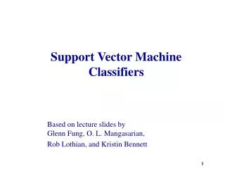
18. Linear Discriminant Functions • 2-class problem • y(x) > 0 : Decide for class C1, else for class C2 • In the following, we focus on linear discriminant functions • If a data set can be perfectly classified by a linear discriminant, then we call it linearly separable. weight vector “bias”(= threshold) B. Leibe Slide credit: Bernt Schiele

19. Linear Discriminant Functions • Decision boundary defines a hyperplane • Normal vector: • Offset: B. Leibe Slide credit: Bernt Schiele

20. Linear Discriminant Functions • Notation • D : Number of dimensions with constant B. Leibe Slide credit: Bernt Schiele

21. Extension to Multiple Classes • Two simple strategies • How many classifiers do we need in both cases? • What difficulties do you see for those strategies? One-vs-all classifiers One-vs-one classifiers B. Leibe Image source: C.M. Bishop, 2006

22. Extension to Multiple Classes • Problem • Both strategies result in regions for which the pure classification result (yk> 0) is ambiguous. • In the one-vs-all case, it is still possible to classify those inputs based on thecontinuous classifier outputs yk > yj8jk. • Solution • We can avoid those difficulties by takingK linear functions of the formand defining the decision boundaries directlyby deciding for Ck iff yk > yj8jk. • This corresponds to a 1-of-K coding scheme B. Leibe Image source: C.M. Bishop, 2006

23. Extension to Multiple Classes • K-class discriminant • Combination of K linear functions • Resulting decision hyperplanes: • It can be shown that the decision regions of such a discriminant are always singly connected and convex. • This makes linear discriminant models particularly suitable for problems for which the conditional densities p(x|wi) are unimodal. B. Leibe Image source: C.M. Bishop, 2006

24. Topics of This Lecture • Linear discriminant functions • Definition • Extension to multiple classes • Least-squares classification • Derivation • Shortcomings • Generalized linear models • Connection to neural networks • Generalized linear discriminants & gradient descent B. Leibe

25. General Classification Problem • Classification problem • Let’s consider K classes described by linear models • We can group those together using vector notationwhere • The output will again be in 1-of-K notation.  We can directly compare it to the target value . B. Leibe

26. General Classification Problem • Classification problem • For the entire dataset, we can writeand compare this to the target matrix T where • Result of the comparison: Goal: Choose suchthat this is minimal! B. Leibe

27. Least-Squares Classification • Simplest approach • Directly try to minimize the sum-of-squares error • We could write this as • But let’s stick with the matrix notation for now… B. Leibe

28. Least-Squares Classification using: • Simplest approach • Directly try to minimize the sum-of-squares error • Taking the derivative yields chain rule: using: B. Leibe

29. Least-Squares Classification • Minimizing the sum-of-squares error • We then obtain the discriminant function as  Exact, closed-form solution for the discriminant function parameters. “pseudo-inverse” B. Leibe

30. Problems with Least Squares • Least-squares is very sensitive to outliers! • The error function penalizes predictions that are “too correct”. B. Leibe Image source: C.M. Bishop, 2006

31. Problems with Least-Squares • Another example: • 3 classes (red, green, blue) • Linearly separable problem • Least-squares solution:Most green points are misclassified! • Deeper reason for the failure • Least-squares corresponds to Maximum Likelihood under the assumption of a Gaussian conditional distribution. • However, our binary target vectors have a distribution that is clearly non-Gaussian!  Least-squares is the wrong probabilistic tool in this case! B. Leibe Image source: C.M. Bishop, 2006

32. Topics of This Lecture • Linear discriminant functions • Definition • Extension to multiple classes • Least-squares classification • Derivation • Shortcomings • Generalized linear models • Connection to neural networks • Generalized linear discriminants & gradient descent B. Leibe

33. Generalized Linear Models • Linear model • Generalized linear model • g(¢ ) is called an activation function and may be nonlinear. • The decision surfaces correspond to • If g is monotonous (which is typically the case), the resulting decision boundaries are still linear functions of x. B. Leibe

34. Generalized Linear Models • Consider 2 classes: with B. Leibe Slide credit: Bernt Schiele

35. Logistic Sigmoid Activation Function Example: Normal distributionswith identical covariance B. Leibe Slide credit: Bernt Schiele

36. Normalized Exponential • General case of K > 2 classes: • This is known as the normalized exponential or softmax function • Can be regarded as a multiclass generalization of the logistic sigmoid. with B. Leibe Slide credit: Bernt Schiele

37. Relationship to Neural Networks • 2-Class case • Neural network (“single-layer perceptron”) with constant B. Leibe Slide credit: Bernt Schiele

38. Relationship to Neural Networks • Multi-class case • Multi-class perceptron with constant B. Leibe Slide credit: Bernt Schiele

39. Logistic Discrimination • If we use the logistic sigmoid activation function… … then we can interpret the y(x) as posterior probabilities! B. Leibe Slide adapted from Bernt Schiele

40. Other Motivation for Nonlinearity • Recall least-squares classification • One of the problems was that datapoints that are “too correct” have a strong influence on the decisionsurface under a squared-error criterion. • Reason: the output of y(xn;w) can grow arbitrarily large for some xn: • By choosing a suitable nonlinearity (e.g.a sigmoid), we can limit those influences B. Leibe

41. Discussion: Generalized Linear Models • Advantages • The nonlinearity gives us more flexibility. • Can be used to limit the effect of outliers. • Choice of a sigmoid leads to a nice probabilistic interpretation. • Disadvantage • Least-squares minimization in general no longer leads to a closed-form analytical solution.  Need to apply iterative methods.  Gradient descent. B. Leibe

42. Linear Separability • Up to now: restrictive assumption • Only consider linear decision boundaries • Classical counterexample: XOR B. Leibe Slide credit: Bernt Schiele

43. Linear Separability • Even if the data is not linearlyseparable, a linear decision boundary may still be “optimal”. • Generalization • E.g. in the case of Normal distributeddata (with equal covariance matrices) • Choice of the right discriminant function is important and should be based on • Prior knowledge (of the general functional form) • Empirical comparison of alternative models • Linear discriminants are often used as benchmark. B. Leibe Slide credit: Bernt Schiele

44. Generalized Linear Discriminants • Generalization • Transform vector x with M nonlinear basis functions Áj(x): • Purpose of Áj(x): basis functions • Allow non-linear decision boundaries. • By choosing the right Áj, every continuous function can (in principle) be approximated with arbitrary accuracy. • Notation with B. Leibe Slide credit: Bernt Schiele

45. Generalized Linear Discriminants • Model • K functions (outputs) yk(x;w) • Learning in Neural Networks • Single-layer networks: Áj are fixed, only weights w are learned. • Multi-layer networks: both the w and the Áj are learned. • In the following, we will not go into details about neural networks in particular, but consider generalized linear discriminants in general… B. Leibe Slide credit: Bernt Schiele

46. Gradient Descent • Learning the weights w: • N training data points: X = {x1, …, xN} • K outputs of decision functions: yk(xn;w) • Target vector for each data point: T= {t1, …, tN} • Error function (least-squares error) of linear model B. Leibe Slide credit: Bernt Schiele

47. Gradient Descent • Problem • The error function can in general no longer be minimized in closed form. • ldea (Gradient Descent) • Iterative minimization • Start with an initial guess for the parameter values . • Move towards a (local) minimum by following the gradient. • This simple scheme corresponds to a 1st-order Taylor expansion (There are more complex procedures available). ´: Learning rate B. Leibe

48. Gradient Descent – Basic Strategies • “Batch learning” • Compute the gradient based on all training data: ´: Learning rate B. Leibe Slide credit: Bernt Schiele

49. Gradient Descent – Basic Strategies • “Sequential updating” • Compute the gradient based on a single data point at a time: ´: Learning rate B. Leibe Slide credit: Bernt Schiele

50. Gradient Descent • Error function B. Leibe Slide credit: Bernt Schiele