Download

1 / 19
190 likes | 195 Views
Explore the concepts of the Traveling Salesman Problem (TSP), Vehicle Routing Problem (VRP), and their impact on transportation logistics. Learn about approximation methods and tailored strategies to optimize delivery routes. Understand the principles of user equilibrium (UE) and system optimal (SO) solutions.

E N D
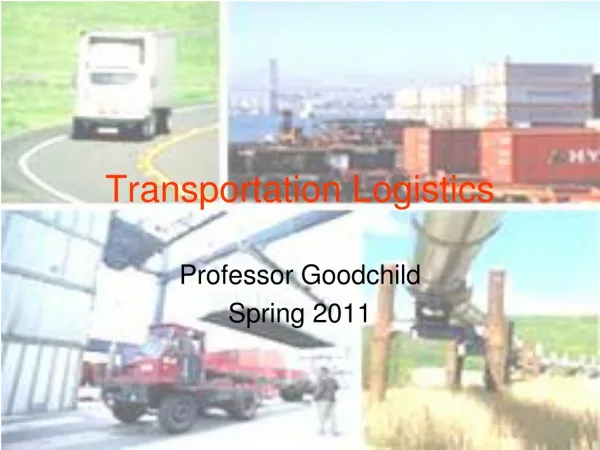
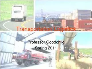
Transportation Logistics Professor Goodchild Spring 2009
Traveling Salesman Problem • Visit a set of cities and minimize total travel cost • Applies to delivery routes • Assume travel costindependent of order • Individual traveler
Traveling Salesman Problem • Can be formulated as an integer programming problem • The time to find an optimal solution increases very quickly with N • Requires location of each city (customer) to be visited
TSP approximation • Is there a formula for L* (the optimum expected length) if N points are randomly scattered (with density δ) in a square region of area A? • L*~k √(AN)=kN/√δ • k depends on the metric (approximately 0.72 for L2 (Euclidean), .92 for L1 (grid)) • Works well for large N • Other formulae for different shapes, moderate N
Vehicle Routing Problem • Assume given locations of N points, a depot, a matrix of costs to travel between locations, a demand for each point, a vehicle capacity • Find an allocation of points to vehicles and a set of vehicle routes ending and beginning at the depot that minimizes either vehicle distance, number of vehicles, or a combination of the two • Assumes number of vehicles known
VRP • Can be formulated as an integer program in a variety of ways • The time to find an optimal solution increases very quickly with N • Faster solution methods have been developed that don’t find the optimum but find a good solution • Local search methods (simulated annealing)
TSP approximation • r: distance from depot to center of tour area • D: total demand (units) • vm: vehicle capacity • Lvrp≤Ltsp+2Dr/vm
Time windows • A time window is an interval in time, provided for the delivery of some good • A narrow time window is a short one, say 30 minutes in length • A wide time window is a long one, say 8 hours in length • How do time windows effect the vehicle routing problem?
Questions • How does the length of a tour change with demand density? • How does the number of drivers change with the length of a tour? • How would you calculate the demand density with 30 minute time windows versus 2 hour time windows?
Tailored Strategies • Tighter time windows for customers that are willing to pay more. • Deliveries outside of peak travel periods. • Allow transportation companies to expand their markets. • Increase logistical complexity.
Wardrop’s First Principal • The journey times in all routes actually used are equal and less than those which would be experienced by a single vehicle on any unused route. • Each user non-cooperatively seeks to minimize his cost of transportation. • Referred to as "user equilibrium" (UE) flows. • User-optimized equilibrium is reached when no user may lower his transportation cost through unilateral action.
Wardrop’s Second Principal • At equilibrium the average journey time is minimum. • This implies that each user behaves cooperatively in choosing his own route to ensure the most efficient use of the whole system. • Referred to as "system optimal" (SO). • Economists argue this can be achieved with marginal costroad pricing.
D1 Link 1 Flow = X1 Cost = Z1 Link 3 Flow = X3 Cost = X3 O Link 2 Flow = X2 Cost = Z2 D2 • Given OD flow from O to D2 is 4 • Choose fraction of flow to travel link 1 and 3 or link 2 • Identify UE solution, SO solution
D1 Link 1 Flow = X1 Cost = Z1 Link 3 Flow = X3 Cost = X3 O Link 2 Flow = X2 Cost = Z2 D2 X1=4(1+x), X2=4(1-x), X3=4x x is fraction of items for D2 sent through D1 Z1=1/X1, Z2=X2, Z3=1 Total Cost = X1Z1+X2Z2+X3Z3 UE: travel cost on both links equivalent SO: minimize total travel cost
D1 Link 1 Flow = X1 Cost = Z1 Link 3 Flow = X3 Cost = X3 O Link 2 Flow = X2 Cost = Z2 D2 UE: x=.7 SO: x=.5
D1 Link 1 Flow = X1 Cost = Z1 Link 3 Flow = X3 Cost = X3 O Link 2 Flow = X2 Cost = Z2 D2 X1=4(1+x), X3=4x, X2=4(1-x) Z1=X1-1/2, Z2=3X2-1/2, Z3=1 Total Cost = X1Z1+X2Z2+X3Z3 Total Cost = 2(1+x)1/2+6(1-x)1/2+4x
X1=4(1+x), X3=4x, X2=4(1-x) Total Cost = X1Z1+X2Z2+X3Z3 Z1=X1-1/2, Z2=3X2-1/2, Z3=1 Total Cost = 2(1+x)1/2+6(1-x)1/2+4x Higher the flow, lower the per unit cost – economy of scale Which links have economies of scale?
Total cost minimized at x=1 Total cost = 6.8 Total cost x Want to send everything on the same route