Download
1 / 123
1.23k likes | 1.26k Views
Introduction to Deep Learning. Data Science International Summer School Predeal August 26, 2018. Razvan C. Bunescu School of Electrical Engineering and Computer Science http://ace.cs.ohio.edu/~razvan bunescu@ohio.edu. Outline. Representation Learning. Feedforward Neural Networks:

E N D
Introduction to Deep Learning Data Science International Summer School Predeal August 26, 2018 Razvan C. Bunescu School of Electrical Engineering and Computer Science http://ace.cs.ohio.edu/~razvan bunescu@ohio.edu
Outline • Representation Learning. • Feedforward Neural Networks: • Fully Connected Networks. • Universal Approximation Theorem. • Forward and Backward Propagation. • Depth is Important • Convolutional Neural Networks. • Recurrent Neural Networks. • Neural Attention. Lecture 01
The Importance of Representation http://www.deeplearningbook.org Lecture 01
From Cartesian to Polar Coordinates • Manually engineered: (first quadrant) • Learned from data: logistic neuron x … y p(blue|x,y) fixed to 1 Fully connected layers: linear transformation W + element-wise nonlinearity f => f(Wx) Lecture 01
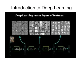
Representation Learning: Images https://www.datarobot.com/blog/a-primer-on-deep-learning/
Representation Learning: Images https://www.datarobot.com/blog/a-primer-on-deep-learning/ Lecture 01
Representation Learning: Text https://www.tensorflow.org/tutorials/word2vec Lecture 01
Representation Learning: Text https://www.tensorflow.org/tutorials/word2vec • Word embeddings, projected 2D through PCA: Lecture 01
Machine Translation https://research.googleblog.com/2016/09/a-neural-network-for-machine.html • Japanese to English: which is human, which is machine? • Kilimanjaro is a snow-covered mountain 19,710 feet high, and is said to be the highest mountain in Africa. Its western summit is called the Masai “Ngaje Ngai,” the House of God. Close to the western summit there is the dried and frozen carcass of a leopard. No one has explained what the leopard was seeking at that altitude. • Kilimanjaro is a mountain of 19,710 feet covered with snow and is said to be the highest mountain in Africa. The summit of the west is called “Ngaje Ngai” in Masai, the house of God. Near the top of the west there is a dry and frozen dead body of leopard. No one has ever explained what leopard wanted at that altitude. Lecture 01
Machine Translation https://research.googleblog.com/2016/09/a-neural-network-for-machine.html • From Phrase-Based Machine Translation (PBMT) to Neural Machine Translation (NMT): Lecture 01
Machine Translation http://www.nytimes.com/2016/12/14/magazine/the-great-ai-awakening.html Uno no es lo que es por lo que escribe, sino por lo que ha leído. • Before November 2016: • One is not what is for what he writes, but for what he has read. • After November 2016: • You are not what you write, but what you have read. Lecture 01
Machine Translation http://www.nytimes.com/2016/12/14/magazine/the-great-ai-awakening.html • Before November 2016: • Kilimanjaro is 19,710 feet of the mountain covered with snow, and it is said that the highest mountain in Africa. Top of the west, “Ngaje Ngai” in the Maasai language, has been referred to as the house of God. The top close to the west, there is a dry, frozen carcass of a leopard. Whether the leopard had what the demand at that altitude, there is no that nobody explained. • After November 2016: • Kilimanjaro is a mountain of 19,710 feet covered with snow and is said to be the highest mountain in Africa. The summit of the west is called “Ngaje Ngai” in Masai, the house of God. Near the top of the west there is a dry and frozen dead body of leopard. No one has ever explained what leopard wanted at that altitude. Lecture 01
Why Deep Learning so Successful? • Large amounts of (labeled) data: • Performance improves with depth. • Deep architectures need more data. • Faster computation: • Originally, GPUs for parallel computation. • Google’s specialized TPUs for TensorFlow. • Microsoft’s generic FPGAs for CNTK. • https://www.microsoft.com/en-us/research/blog/microsoft-unveils-project-brainwave/ • Better algorithms and architectures. Lecture 01
A Rapidly Evolving Field • Used to think that training deep networks requires greedy layer-wise pretraining: • Unsupervised learning of representations with auto-encoders (2012). • Better random weight initialization schemes now allow training deep networks from scratch. • Batch normalization allows for training even deeper models (2014). • Residual learning allows training arbitrarily deep networks (2015). Lecture 01
Feedforward Neural Networks • Fully Connected Networks. • Universal Approximation Theorem • Convolutional Neural Networks Lecture 01
Universal Approximation Theorem Hornik (1991), Cybenko (1989) • Let σ be a nonconstant, bounded, and monotonically-increasing continuous function; • Let Im denote the m-dimensional unit hypercube [0,1]m; • Let C(Im) denote the space of continuous functions on Im; • Theorem: Given any function f C(Im) and ε > 0, there exist an integer N and real constants αi, bi R, wi Rm, where i = 1, ..., N, such that: where Lecture 02
Universal Approximation Theorem Hornik (1991), Cybenko (1989) x1 wi1 σ wi2 αi x2 σ Σ wi3 x3 σ bi +1 +1 Lecture 02
Polynomials as Simple NNs [Lin & Tegmark, 2016] Lecture 12
Neural Network Model • Put together many neurons in layers, such that the output of a neuron can be the input of another: input layer hidden layer output layer Lecture 02
input features x bias units • nl =3 is the number of layers. • L1 is the input layer, L3 is the output layer • (W, b) = (W(1), b(1), W(2), b(2)) are the parameters: • W(l)ij is the weight of the connection between unit j in layer l and unit i in layer l + 1. • b(l)i is the bias associated unit unit i in layer l + 1. • a(l)i is the activationof unit i in layer l, e.g. a(1)i = xi and a(3)1 = hW,b(x). Lecture 02
Inference: Forward Propagation • The activations in the hidden layer are: • The activations in the output layer are: • Compressed notation: where Lecture 02
Forward Propagation • Forward propagation (unrolled): • Forward propagation (compressed): • Element-wise application: • f(z) = [f(z1), f(z2), f(z3)] Lecture 02
Forward Propagation • Forward propagation (compressed): • Composed of two forward propagation steps: Lecture 02
Multiple Hidden Units, Multiple Outputs • Write down the forward propagation steps for: Lecture 02
Learning: Backpropagation • Regularized sum of squares error: • Gradient: +1 ? Lecture 02
Backpropagation • Need to compute the gradient of the squared error with respect to a single training example (x, y): Lecture 02
Univariate Chain Rule for Differentiation • Univariate Chain Rule: • Example: Lecture 02
Multivariate Chain Rule for Differentiation • Multivariate Chain Rule: • Example: Lecture 02
Backpropagation: • J depends on Wij(l)only through ai(l+1), which depends on Wij(l)only through zi(l+1). ... Lecture 02
Backpropagation: • J depends on bi(l)only through ai(l+1), which depends on bi(l)only through zi(l+1). J ... +1 Lecture 02
Backpropagation: and How to compute for all layers l ? +1 Lecture 02
Backpropagation: • J depends on ai(l)only through a1(l+1), a2(l+1), ... ? J ... Lecture 02
Backpropagation: • J depends on ai(l)only through a1(l+1), a2(l+1), ... • Therefore, can be computed as: Lecture 02
Backpropagation: • Start computing δ’s for the output layer: Lecture 02
Backpropagation Algorithm • Feedforward pass on x to compute activations • For each output unit i compute: • For l = nl−1, nl−2, nl−3, ..., 2 compute: • Compute the partial derivatives of the cost Lecture 02
Backpropagation Algorithm: Vectorization for 1 Example • Feedforward pass on x to compute activations • For last layer compute: • For l = nl−1, nl−2, nl−3, ..., 2 compute: • Compute the partial derivatives of the cost Lecture 02
Backpropagation Algorithm: Vectorization for Dataset of m Examples • Feedforward pass on X to compute activations • For last layer compute: • For l = nl−1, nl−2, nl−3, ..., 2 compute: • Compute the partial derivatives of the cost /m .col_avg() Lecture 02
Backpropagation: Softmax Regression • Consider layer nl to be the input to the softmax layer i.e. softmax output layer is nl+1. Softmax output Softmax input Softmax weights Cross-entropy ...
Backpropagation: Softmax Regression • Consider layer nl to be the input to the softmax layer i.e. softmax output layer is nl+1. • Softmax weights stored in matrix . • K classes => Lecture 02
Backpropagation Algorithm: Softmax (1) • Feedforward pass on x to compute activations for layers l = 1, 2, …, nl. • Compute softmax outputs and objective . • Let T be the one-hot vector representation for label y. • Compute gradient with respect to softmax weights: Lecture 02
Backpropagation Algorithm: Softmax (2) • Compute gradient with respect to softmax inputs: • For l = nl−1, nl−2, nl−3, ..., 2 compute: • Compute the partial derivatives of the cost
Backpropagation Algorithm: Softmax for 1 Example • For softmax layer, compute: • For l = nl, nl−2, nl−3, ..., 2 compute: • Compute the partial derivatives of the cost one-hot label vector
Backpropagation Algorithm: Softmax for Dataset of m Examples • For softmax layer, compute: • For l = nl, nl−1, nl−2, ..., 2 compute: • Compute the partial derivatives of the cost ground-truth label matrix /m .col_avg()
Backpropagation: Logistic Regression Lecture 02
Shallow vs. Deep Networks • A 1-hidden layer network is a fairly shallow network. • Effective for MNIST, but limited by simplicity of features. • A deep network is a k-layer network, k > 1. • Computes more complex features of the input, as k gets larger. • Each hidden layer computes a non-linear transformation of the previous layer. Conjecture A deep network has significantly greater representational power than a shallow one. Lecture 12
Deep vs. Shallow Architectures • A function is highly varying when a piecewise (linear) approximation would require a large number of pieces. • Depth of an architecture refers to the number of levels of composition of non-linear operations in the function computed by the architecture. • Conjecture: Deep architectures can compactly represent highly-varying functions: • The expression of a function is compactwhen it has few computational elements. • Same highly-varying functions would require very large shallow networks. Lecture 12
Graphs of Computations • A function can be expressed by the composition of computational elements from a given set: • logic operators. • logistic operators. • multiplication and additions. • The function is defined by a graph of computations: • A directed acyclic graph, with one node per computational element. • Depth of architecture = depth of the graph = longest path from an input node to an output node. Lecture 12
Functions as Graphs of Computations [Bengio, FTML’09] Lecture 12
Polynomials as Graphs of Computations [Bengio, FTML’09] Lecture 12
Sum-Product Networks (SPNs) [Poon & Domingos, UAI’11] • Rooted, weighted DAG. • Nodes: Sum, Product, (Input) Indicators. • Weights on edgesfrom sums to children. Lecture 12