Download
1 / 26
260 likes | 341 Views
A High Latitude Source for Outer Radiation Belt Electrons?. Robert Sheldon September 23, 2004 National Space Science & Technology Center. Motivation.

E N D
A High Latitude Source for Outer Radiation Belt Electrons? Robert Sheldon September 23, 2004 National Space Science & Technology Center
Motivation • POLAR and CLUSTER have discovered keV-MeV ions and electrons permanently trapped * in the quadrupolar outer cusp region*. The Quadrupole trap, just like the Dipole trap, has min/max limits on energy, pitchangle and “L-shell” (we call “C-shell”)*. Minimum energy is defined by “separatrix” energy (ExB = B). The max energy defined by rigidity. • Mapping C-shell limits to the dipole give 5<L<∞. very close to the PSD “bump” • Mapping Quad Energy limits to the rad belts, give ~ 0-50 keV for protons, and 1-10 MeV for electrons. • Mapping pitchangles give 0o < a < 50omicroburst? • Q: How would this reservoir be connected to ORBE?
Sheldon et al., GRL 1998 POLAR/ CAMMICE data 1 MeV electron PSD in outer cusp
QuadrupolarT87 Magnetosphere • Since Chapman & Ferraro 1937, we’ve known the magnetosphere is a quadrupole. • All trapping models have assumed a dipole. • If Quadrupole is source, how does it change the transport?
The Simulated T96 Quadrupole Trap • Lousy Trap • Great Accelerator • Can be made to trap better though.
Outline • Defining the Source vs. Transport Problem • Details of the Transport • Phase Space Compression • Radial diffusion: 6 dimensions 3-D • UBK: 6-D 4-D • ODE vs PDE • Details of the Source • The Dipole Trap • The Quadrupole Trap • Combining UBK + PDE + Quadrupole Transport
Source versus Transport • Making an analogy to $, “Did he make that money or inherit it?”, separating the neuveau-riche in England “He’s the sort of person who had to buy his silver.” Why is this important? Prediction. Old money acts different than new. • Example: Williams, Frank & Shelley peak seen in ISEE-3 data (35 keV protons). Local acceleration or transport?
Prediction Problems • If ORBE are due to local acceleration then: • What are the energy sources? • What are the optimal conditions? • What are the preconditioning factors? • If ORBE are due to transport then: • What are the reservoirs? • What are the transport coefficients? • What are the preconditioning (storage) factors? • In Summary: The questions we ask of the data are completely different for the two models.
Monte Carlo Integration • What do we want to predict? S/C fluences. • What does particle tracing give us? Single particle transport, f(x,y,z,x’,y’,z’) • How do we get fluences? Integrate over energy, pitchangle, MLT, radius [gyrophase, bounce phase] • How many particles to do this integration? • Monte Carlo methods: sample parameter space evenly • Two drawbacks of Monte Carlo (Press, p. 299): • Smoothness—sample spacing defined by smallest feature • Dimensions—error in solution goes as N-1/2*D10%=1012!
Phase Space Compression • If we can reduce the number of dimensions, then Monte Carlo integration starts to look reasonable. 6D4D = 108 <<1012 for 10% accuracy. • Adiabatic invariants are equivalently integrals over some canonical dimension. • 1st =magnetic moment = GYRO • 2nd=J (“pitchangle”) = BOUNCE • 3rd=L-shell = DRIFT • Thus radial diffusion is 6 - 3 = 3-D calculation. Gyrokinetic = 6 - 1 = 5-D calculation.
Particle tracing Vx,Vy,Vz, X,Y,Z m, J, L, Fm,FJ,FL m,J, L,Fm, FJ,FL,t Vx,Vy,Vz, X,Y,Z,t Radial diffusion B-L space m, J, L m, J, L, t Salammbo Non-MHD Inner M’sphere b<<1 6-D 5-D 4-D 3D • Gyro-kinetic • m, J, L, FJ, FL • m, J, L, FJ, FL,t • Guiding center • m,J,L,FL • m,U,B,K • m,U,B,K,t Dynamic, time-dependent models
Lagrange vs Hamilton • So we can simplify our equations if we use adiabatic (=constant energy) invariants. • From classical mechanics, we can recast the equations of motion either as (x,v) or (E,t). Numerically, Lagrangian solvers include time explicitly x = f(t), and energy is implicit, whereas Hamiltonian solvers include energy explicitly, time implicit x = f(E). Adiabats beg for Hamilton. • Accelerator designers find Hamiltonian methods converge faster to higher accuracy. (MaryLIE)
What kind of Transport Code? • Einstein: “As simple as possible but no simpler” Lowest dimensionality possible by considering time- and spatial- scales required for solution. • Hamilton-Jacobi theory for set of action-angle variables with best convergence properties. • Coupled PDE with appropriate diffusion coefficients, preferably diagonalized • Flowfield separation of diffusion from convection to allow operator splitting.
PDE vs ODE • BUT many processes are not purely adiabatic, they DIFFUSE. How is this handled? • Lagrangian ODE tracing can be done for many different magnetospheric conditions, and averaged over that as well. Equivalent to adding a 7th additional time dimension. • Hamiltonian adiabatic methods have already averaged over some temporal scales implicitly. Non-adiabatic behavior introduces 2nd order cross terms (diffusion) into the system, equivalent to going from ODE PDE with the same number of dimensions. Now one uses PDE not MonteCarlo integration. Time is implicit, so careful attention must be spent splitting the diffusion timescale from the convection timescale, or else the PDE solves the wrong problem. • Choice of appropriate coordinates is CRITICAL for PDE.
If coordinates are not separable, ==>new physics: Vortices, convection Anomalous, or enhanced diffusion, “migration” Convection + diffusion = confusion If coordinates are separable, then D = D1 * D2 ==> diagonally dominant, easily generalized from 1-D. DLL, Daa, Dmm ==> radial diffusion models (Schulz 74) 2D+ Diffusive Transport Is there a coordinate system which is separable?
The Dipole Trap • Great Trap • Lousy accelerator • Source of E >1 keV particles outside trap. Where?
Quadrupole Trap in the Laboratory(Two 1-T magnets, -400V, 50mTorr)
4-D UBK Hamiltonian • The Quadrupole trap is located at a specific MLT as well as high-latitude. Thus we need to keep the 3rd invariant phase4-D • We use two, energy conserving, 4D coordinate systems: • ƒ1(M,K,U,Bm,n,t): “radial” diffusion + convection • ƒ2(T,a,n,X,Y,t): Coulomb collisions + pitchangle diffusion • Where “n” separates quadrupole & dipole trapping • Operator splitting enables us to carry out radial transport on ƒ1, and pitchangle+energy loss on ƒ2.
PDE Diffusion Equation • dfk/dt= ∂fk/∂t+ C∂f/∂y+ Dz∂2fk/∂z2+ ∂/∂xi(Dij ∂fk/∂xj) • i,j= index for (M,K) or (E,a); k = quad or dipole trap • 1st term is the source + loss terms • 2nd term is convective velocity in (U,Bm)-space • 3rd term is diffusion in (U,Bm)-space • 4th term is remaining diffusion in (E,a)-space • Mixed parabolic & elliptic PDE solved with standard finite element techniques. Operator splitting, mapping between ƒ1 ƒ2 (Fast, efficient, not numerically diffusive).
Conclusions • The UBK transform has the unique property of solving several requirements at once: • Separates convection from diffusion (MLT-dependence) • Permits Hamilton-Jacobi solution to equations of motion • Treats both Quadrupole & Dipole Regions (hi-latitudes) • Permits rapid calculation of diffusion coefficients • Can use operator splitting to diagonalize Diffusion tensor • Cannot handle time- or spatial- scales that violate 1st invariant. E.g. rare shock acceleration events (1991). • It should indicate whether a hi-latitude source exists.
Implications • ORBITALS should have instruments with sufficient resolution of energy and pitchangle (T,a) to resolve the transport of this very small region of parameter space as it would look when mapped to the equator. Pitchangle resolution < 5o, spatial (temporal) resolution < 1o.at the appropriate energies.