Download
1 / 38
380 likes | 530 Views
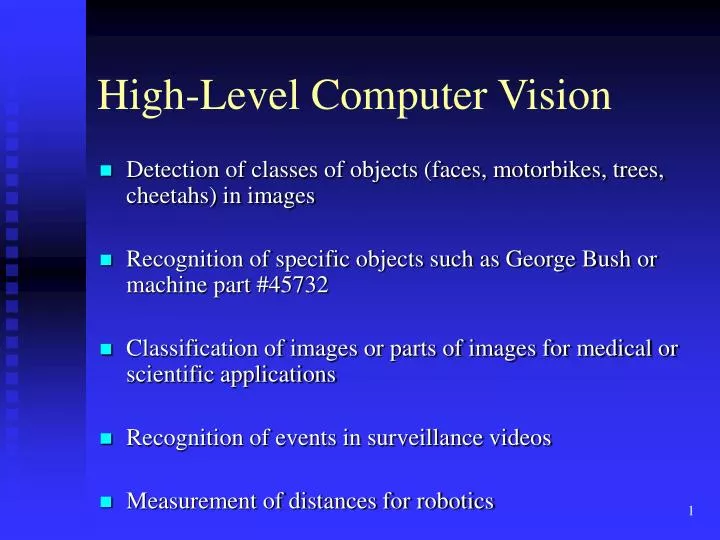
High-Level Computer Vision. Detection of classes of objects (faces, motorbikes, trees, cheetahs) in images Recognition of specific objects such as George Bush or machine part #45732 Classification of images or parts of images for medical or scientific applications

E N D
High-Level Computer Vision • Detection of classes of objects (faces, motorbikes, trees, cheetahs) in images • Recognition of specific objects such as George Bush or machine part #45732 • Classification of images or parts of images for medical or scientific applications • Recognition of events in surveillance videos • Measurement of distances for robotics
High-level vision uses techniques from AI. • Graph-Matching: A*, Constraint Satisfaction, Branch and Bound Search, Simulated Annealing • Learning Methodologies: Decision Trees, Neural Nets, SVMs, EM Classifier • Probabilistic Reasoning, Belief Propagation, Graphical Models
Graph Matching for Object Recognition • For each specific object, we have a geometric model. • The geometric model leads to a symbolic model in terms of image features and their spatial relationships. • An image is represented by all of its features and their spatial relationships. • This leads to a graph matching problem.
Model-based Recognition as Graph Matching • Let U = the set of model features. • LetR be a relation expressing their spatial relationships. • LetL = the set of image features. • Let S be a relation expressing their spatial relationships. • The ideal solution would be a subgraph isomorphism f: U-> L satisfying • if (u1, u2, ..., un) R, then (f(u1),f(u2),...,f(un)) S
House Example 2D model 2D image P L RP and RL are connection relations. f(S1)=Sj f(S2)=Sa f(S3)=Sb f(S4)=Sn f(S5)=Si f(S6)=Sk f(S10)=Sf f(S11)=Sh f(S7)=Sg f(S8) = Sl f(S9)=Sd
But this is too simplistic • The model specifies all the features of the object that may appear in the image. • Some of them don’t appear at all, due to occlusion or failures at low or mid level. • Some of them are broken and not recognized. • Some of them are distorted. • Relationships don’t all hold.
TRIBORS: view class matching of polyhedral objects edges from image model overlayed improved location • A view-class is a typical 2D view of a 3D object. • Each object had 4-5 view classes (hand selected). • The representation of a view class for matching included: • - triplets of line segments visible in that class • - the probability of detectability of each triplet • The first version of this program used depth-limited A* search.
RIO: Relational Indexing for Object Recognition • RIO worked with more complex parts that could have • - planar surfaces • - cylindrical surfaces • - threads
Object Representation in RIO • 3D objects are represented by a 3D mesh and set of 2D view classes. • Each view class is represented by an attributed graph whose • nodes are features and whose attributed edges are relationships. • For purposes of indexing, attributed graphs are stored as • sets of 2-graphs, graphs with 2 nodes and 2 relationships. share an arc coaxial arc cluster ellipse
RIO Features ellipses coaxials coaxials-multi parallel lines junctions triples close and far L V Y Z U
RIO Relationships • share one arc • share one line • share two lines • coaxial • close at extremal points • bounding box encloses / enclosed by
Hexnut Object How are 1, 2, and 3 related? What other features and relationships can you find?
Graph and 2-Graph Representations 1 coaxials- multi encloses 1 1 2 3 2 3 3 2 encloses 2 ellipse e e e c encloses 3 parallel lines coaxial
Relational Indexing for Recognition Preprocessing (off-line) Phase • for each model view Mi in the database • encodeeach 2-graph of Mi to produce an index • store Mi and associated information in the indexed • bin of a hash table H
Matching (on-line) phase • Construct a relational (2-graph) description D for the scene • For each 2-graph G of D • Select the Mis with high votes as possible hypotheses • Verify or disprove via alignment, using the 3D meshes • encode it, producing an index to access the hash table H • cast a vote for each Mi in the associated bin
RIO Verifications incorrect hypothesis 1. The matched features of the hypothesized object are used to determine its pose. 2. The 3D mesh of the object is used to project all its features onto the image. 3.A verification procedure checks how well the object features line up with edges on the image.
Use of classifiers is big in computer vision today. • 2 Examples: • Rowley’s Face Detection using neural nets • Our 3D object classification using SVMs
Object Detection: Rowley’s Face Finder 1.convert to gray scale 2. normalize for lighting 3. histogram equalization 4. apply neural net(s) trained on 16K images What data is fed to the classifier? 32 x 32 windows in a pyramid structure
3D-3D Alignment of Mesh Models to Mesh Data • Older Work: match 3D features such as 3D edges and junctions • or surface patches • More Recent Work: match surface signatures - curvature at a point - curvature histogram in the neighborhood of a point - Medioni’s splashes - Johnson and Hebert’s spin images *
The Spin Image Signature P is the selected vertex. X is a contributing point of the mesh. is the perpendicular distance from X to P’s surface normal. is the signed perpendicular distance from X to P’s tangent plane. X n tangent plane at P P
Spin Image Construction • A spin image is constructed • - about a specified oriented point oof the object surface • - with respect to a set of contributing points C, which is • controlled by maximum distance and angle from o. • It is stored as an array of accumulators S(,) computed via: • For each point cin C(o) • 1. compute and for c. • 2. increment S (,) o
Spin Image Matching ala Sal Ruiz
+ Sal Ruiz’s Classifier Approach Numeric Signatures 1 Components 2 4 Architecture of Classifiers Recognition And Classification Of Deformable Shapes Symbolic Signatures 3
Numeric Signatures: Spin Images 3-D faces P • Rich set of surface shape descriptors. • Their spatial scale can be modified to include local and non-local surface features. • Representation is robust to scene clutter and occlusions. Spin images for point P
… How To Extract Shape Class Components? Training Set Select Seed Points Compute Numeric Signatures Region Growing Algorithm Component Detector … Grown components around seeds
Component Extraction Example Labeled Surface Mesh Selected 8 seed points by hand Region Growing Detected components on a training sample Grow one region at the time (get one detector per component)
How To Combine Component Information? … 1 1 1 1 2 2 2 2 2 2 2 4 3 5 6 7 8 Extracted components on test samples Note: Numeric signatures are invariant to mirror symmetry; our approach preserves such an invariance.
3 4 5 8 7 6 Symbolic Signature Labeled Surface Mesh Symbolic Signature at P Critical Point P Encode Geometric Configuration Matrix storing component labels
Symbolic Signatures Are Robust To Deformations P 4 3 3 4 3 3 4 3 4 4 5 5 5 5 5 8 8 8 8 8 6 7 6 7 6 7 6 7 6 7 Relative position of components is stable across deformations: experimental evidence
Proposed Architecture(Classification Example) Verify spatial configuration of the components Identify Components Identify Symbolic Signatures Class Label Input Labeled Mesh -1 (Abnormal) Two classification stages Surface Mesh
At Classification Time (1) Labeled Surface Mesh Surface Mesh Multi-way classifier Bank of Component Detectors Assigns Component Labels Identify Components
At Classification Time (2) Labeled Surface Mesh +1 Symbolic pattern for components 1,2,4 1 4 Bank of Symbolic Signatures Detectors Assigns Symbolic Labels 2 5 Two detectors 6 Symbolic pattern for components 5,6,8 8 -1
Architecture Implementation • ALL our classifiers are (off-the-shelf) ν-Support Vector Machines (ν-SVMs) (Schölkopf et al., 2000 and 2001). • Component (and symbolic signature) detectors are one-class classifiers. • Component label assignment: performed with a multi-way classifier that uses pairwise classification scheme. • Gaussian kernel.
Snowman: 93%. Rabbit: 92%. Dog: 89%. Cat: 85.5%. Cow: 92%. Bear: 94%. Horse: 92.7%. Human head: 97.7%. Human face: 76%. Task 1: Recognizing Single Objects (2) Recognition rates (true positives) (No clutter, no occlusion, complete models)
Task 2-3: Recognition in Complex Scenes (2) Task 2 Task 3