Network Layer

1. Computer Networks Network Layer

2. Chapter 4 Outline 4.1 Introduction and Network Service Models 4.2 Routing Principles 4.3 Hierarchical Routing 4.4 Routing in the Internet 4.5 The Internet (IP) Protocol 4.6 What’s Inside a Router 4.7 IPv6 4.8 Multicast Routing 4.9 Mobility

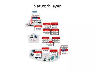
3. transport packet from sending to receiving hosts network layer protocols in every host, router three important functions: path determination: route taken by packets from source to dest. (Routing Algorithms) forwarding: move packets from router’s input to appropriate router output call setup: some network architectures require router call setup along path before data flows network data link physical Network Layer Functions application transport network data link physical application transport network data link physical

4. Q: What service model for “channel” transporting packets from sender to receiver? Services guaranteed bandwidth? preservation of inter-packet timing (no jitter)? loss-free delivery? in-order delivery? congestion feedback to sender? Network Service Model The most important abstraction provided by network layer: virtual circuit or datagram?

5. call setup, teardown for each call before data can flow each packet carries VC identifier (not destination host ID) every router on source-destination path maintains “state” for each passing connection transport-layer connection only involved two end systems Link and router resources (bandwidth, buffers) may be allocated to VC (dedicated resources = predictable service) to get circuit-like performance. “source-to-destination path behaves much like telephone circuit” performance-wise network actions along source-to-destination path Virtual circuits

6. VC implementation • A VC consists of: • path from source to destination • VC numbers, one number for each link along path • entries in forwarding tables in routers along path • Packet belonging to VC carries VC number (rather than destination address) • VC number can be changed on each link. • New VC number comes from forwarding table

7. Incoming interface Incoming VC # Outgoing interface Outgoing VC # 1 12 3 22 2 63 1 18 3 7 2 17 1 97 3 87 … … … … Forwarding table VC number a 22 32 12 3 1 2 Interface number Routers maintain connection state information! Forwarding table in router a

8. used to setup, maintain teardown VC used in ATM, frame-relay, X.25 not used in today’s Internet application transport network data link physical application transport network data link physical Virtual Circuits: Signaling Protocols 6. Receive data 3. Accept call 2. Incoming call 5. Data flow begins 4. Call connected 1. Initiate call

9. no call setup at network layer routers: no state about end-to-end connections no network-level concept of “connection” packets forwarded using destination host address packets between same source-destination pair may take different paths application transport network data link physical application transport network data link physical Datagram networks: the Internet model 2. Receive Data 1. Send Data

10. Network Layer Service Models: Guarantees ? Congestion feedback no (inferred via loss) no congestion no congestion yes no Network Architecture Internet ATM ATM ATM ATM Service Model best effort CBR VBR ABR UBR Bandwidth none constant rate guaranteed rate guaranteed minimum none Loss no yes yes no no Order no yes yes yes yes Timing no yes yes no no CBR: Constant bit rate VBR: Variable bit rate ABR: Available bit rate UBR: Unspecified bit rate • Internet model being extended: Integrated services, Differentiated Services • Chapter 6

11. Internet (Datagram) data exchange among computers “elastic” service, no strict timing req. “smart” end systems (computers) can adapt, perform control, error recovery simple inside “network”, complexity at “edge” many link types different characteristics uniform service is difficult ATM (Virtual Circuit) evolved from telephony human conversation: strict timing, reliability requirements need for guaranteed service “dumb” end systems telephones complexity inside network Datagram or VC Network: why?

12. Network Interface Buffering in IP routers • Buffer size • Space for bursts of packets • Latency Internet Router Router • Dropping packets • When? • What?

13. FIFO Queueing in the Router(Drop Tail) Network Interface • Single queue maintained

14. FIFO Queueing in the Router (Drop Tail) Network Interface • Single queue maintained • Dequeue from head

15. FIFO Queueing in the Router (Drop Tail) Network Interface • Single queue maintained • Dequeue from head • Enqueue at tail

16. FIFO Queueing in the Router (Drop Tail) Network Interface • Single queue maintained • Dequeue from head • Enqueue at tail • When full

17. FIFO Queueing in the Router (Drop Tail) Network Interface • Single queue maintained • Dequeue from head • Enqueue at tail • When full drop arriving packet (drop-tail)

18. Slow Feedback from Drop Tail • Feedback comes when buffer is completely full • … even though the buffer has been filling for a while • Plus, the filling buffer is increasing RTT • … and the variance in the RTT • Might be better to give early feedback • Get one or two flows to slow down, not all of them • Get these flows to slow down before it is too late

19. Queue Management • Performance Degradation in current TCP Congestion Control • Multiple packet loss • Low link utilization • Congestion collapse • The role of the router (i.e., network) • Control congestion effectively with a network • Allocate bandwidth fairly

20. Active Queue Management • Goals: • Better congestion notification for responsive flows (i.e. TCP) • Maintain shorter queues • Fairness in drops (proportional)

21. Random Early Detection (RED) • Invented by Sally Floyd and Van Jacobson in the early 1990s, differs from the DECbit in two major ways • Notification is implicit • just drop the packet (TCP will timeout) • could make explicit by marking the packet • Early random drop • rather than wait for queue to become full, drop each arriving packet with some drop probability whenever the queue length exceeds some drop level

22. Random Early Detection (RED). • Basic idea of RED • Router notices that the queue is getting build-up. • Randomly drops or marks arriving packets (before queue gets full). • Packet drop signals a congestion to the source. • Packet drop probability • Drop probability increases as queue length increases • If buffer is below some level, don’t drop anything • … otherwise, set drop probability as function of queue

23. RED Details • Compute average queue length (Geometric Moving Average) 0 < α < 1 (usually 0.002) SampleLenis queue length each time a packet arrives. MinTh MaxTh SampleLen

24. RED Details. • On arrival of a packet: calculate AvgLen if AvgLen <= MinTh then enqueue arriving packet if MinTh < AvgLen < MaxTh then calculate probability P drop arriving packet with probability P if AvgLen => MaxTh then drop arriving packet

25. RED Details.. • Computing probability P P maxTh minTh 1 maxP AvgLen AvgLen

26. Forced drop Max Threshold Probabilistic drops Min Threshold No drops RED Detail… • Weighted Running Average Queue Length Drop probability Average Queue Length Max Queue Size Time

27. Properties of RED • Drops packets before queue is full • In the hope of reducing the rates of some flows • Drops packet in proportion to each flow’s rate • High-rate flows have more packets • … and, hence, a higher chance of being selected • Drops are spaced out in time • Which should help desynchronize the TCP senders • Tolerant of burstiness in the traffic • By basing the decisions on average queue length

28. Tuning RED • MaxP is typically set to 0.02, meaning that when the average queue size is halfway between the two thresholds, the gateway drops roughly one out of 100 packets. • If traffic isbursty, then MinThreshold should be sufficiently large to allow link utilization to be maintained at an acceptably high level. • Difference between two thresholds should be larger than the typical increase in the calculated average queue length in one RTT; setting MaxThreshold to twiceMinThreshold is reasonable for traffic on today’s Internet.

29. Problems With RED • Hard to get the tunable parameters just right • How early to start dropping packets? • What slope for the increase in drop probability? • What time scale for averaging the queue length? • Sometimes RED helps but sometimes not • If the parameters aren’t set right, RED doesn’t help • And it is hard to know how to set the parameters • RED is implemented in practice • But, often not used due to the challenges of tuning right • Many variations • With cute names like “Blue” and “FRED”…

30. Explicit Congestion Notification • Early dropping of packets • Good: gives early feedback • Bad: has to drop the packet to give the feedback • Explicit Congestion Notification • Router marks the packet with an ECN bit • … and sending host interprets as a sign of congestion • Surmounting the challenges • Must be supported by the end hosts and the routers • Requires two bits in the IP header (one for the ECN mark, and one to indicate the ECN capability) • Solution: borrow two of the Type-Of-Service bits in the IPv4 packet header

31. Chapter 4 Outline 4.1 Introduction and Network Service Models 4.2 Routing Principles • Distance vector routing • Link state routing 4.3 Hierarchical Routing 4.4 Routing in the Internet 4.5 The Internet (IP) Protocol 4.6 What’s Inside a Router 4.7 IPv6 4.8 Multicast Routing 4.9 Mobility

32. The Problem “B” “A” R How does R choose a next-hop on the path towards host B? CS244a Handout 5

33. Interplay between routing, forwarding routing algorithm local forwarding table dest. net. addr. Output port 65/8 128.9/16 128.9.16/20 128.9.19/24 3 2 2 1 dest. IP addr. in arriving packet’s header 1 2 3 128.9.16.14

34. Graph abstraction w x y v z u 5 3 5 2 2 1 3 1 2 Graph: G = (N,E) N = set of routers = { u, v, w, x, y, z } E = set of links ={ (u,v), (u,x), (v,x), (v,w), (x,w), (x,y), (w,y), (w,z), (y,z) } 1 Remark: Graph abstraction is useful in other network contexts Example: P2P, where N is set of peers and E is set of TCP connections

35. Graph abstraction: costs w x y v z u • c(x,x’) = cost of link (x,x’) • e.g., c(w,z) = 5 • cost could always be 1, or inversely related to bandwidth, or inversely related to congestion 5 3 5 2 2 1 3 1 2 1 Cost of path (x1, x2, x3,…, xp) = c(x1,x2) + c(x2,x3) + … + c(xp-1,xp) Question: What’s the least-cost path between u and z ? Routing algorithm: algorithm that finds least-cost path

36. Graph abstraction for routing algorithms: graph nodes are routers graph edges are physical links link cost: Delay (Make high speed links attractive, but closeness counts), $ cost, Inverse of bandwidth, Path utilization(congestion level & queue length), Stability (Is path up or down?) 4 5 3 C B 2 5 3 A 1 2 3 F 1 2 E D 1 Routing protocol Routing Goal: determine “good” path (sequence of routers) thru network from source to dest. Abstract model of a network • “good” path: • typically means minimum cost path • other definitions possible

37. R Technique 1: Naïve Approach Flood!: Routers forward packets to all ports except the input port. • Advantages: • Simple. • Every destination in the network is reachable. • Disadvantages: • Some routers receive a packet multiple times. • Packets can go round in loops forever. • Inefficient. CS244a Handout 5

38. Spanning Trees Objective: Find the lowest cost route from each of (R1, …, R7) to R8. “A” R2 R4 R6 1 1 4 R1 2 3 2 R7 2 R5 R3 3 2 R8 4 “B” CS244a Handout 5

39. A Spanning Tree 1 1 4 R1 2 3 2 R7 2 R5 R3 3 2 R8 4 • The solution is a spanning tree with R8 as the root of the tree. • Tree: There are no loops. • Spanning: All nodes included. • We’ll see two algorithms that build spanning trees automatically: • The distributed Bellman-Ford algorithm ( Distance Vector ). • Dijkstra’s shortest path first algorithm ( Link State ). CS244a Handout 5

40. Routing protocol requirements • Minimizing route table spec: Node memory related issue • Minimizing control message: Overhead in bandwidth • Robustness • Retain its correctness in dynamic situation. Should be free of loops, black holes. • Using optimal paths (optimality) • Choosing the best path ( in terms of some metrics) • Stability: Free of oscillations • Fairness • Should take the complete topology while computing the path • Efficiency: Convergence time • Correctness

41. Design Choices - 1 • Centralized versus Distributed routing • Centralized: One node collects information (node has complete topology and link cost) and then installs the routing information in all nodes (Link state algorithm). • Distributed: All nodes co-operate to form the rooting table. • Source based versushop by hop • Source routing: data packet contains the hop list. • Hop by hop: Each hop takes decision based on its routing table about the next hop (Distance vector algorithm)

42. Design Choices - 2 • Stochasticversusdeterministic • Stochastic: Routing table contains multiple path information. Next hop is chosen randomly. Advantage: load distribution. • Deterministic: always follow same path. • Single versus multiple path • Router can use multiple paths for a single destination • Dynamic versus Static • Dynamic: Routing dependent on the current network state routes update more quickly • periodic update • in response to link cost changes • Static: Routes update slowly over time.

43. Assumptions About Router • Router knows address of each neighbor. • Router can communicate the information with its neighbors. • Router tells its neighbors its best idea of distance to every other router in the network. • Router receives these distance vectorsfrom its neighbors. • Router updates its notion of best path to each destination, and the next hop for this destination.

44. Distance Table Inside Router • Distance Table data structure • row for each possible destination. • column for each directly-attached neighbor router. • example: in router x, for dest. y via neighbor z. • This table is made based on exchanged information about distance metric and calculation. cost to dest. via x D () y y’ y’’ y’’’ z 1 7 6 4 z’ 14 5 9 2 z’ 5 8 4 11 z’ z’’ x z,1 z’,5 z’’,4 z’,4 y’ z y y’’ destination Distance Vector=Routing table y’’’ Distance table in X

45. Routers Information Exchange • Routers exchange information periodically of known: • distance metric (costs) • routing table (distance vector) • Exchange timing: • whenever a link fails • Whenever a routing table entry changes.

46. Iterative: continues until no nodes exchange info. self-terminating: no “signal” to stop Asynchronous: nodes need not exchange info/iterate in lock step! distributed: each node communicates only with directly-attached neighbors Distance Table data structure each node has its own: row for each possible destination column for each directly-attached neighbor to node example: in node X, for dest. Y via neighbor Z: DX(Y,Z) X Z D (Y,Z) c(X,Z) + min {D (Y,w)} = w Distance Vector Routing Algorithm distance from X to Y, via Z as next hop

47. E D(i, j) Distance table: A 1 B 7 A D (A,C) 2 D (A,B)= 8 E C D E B 1 c(E,B) + min {D (A,w)} = D B 2 E 8 + 6 = 14 c(E,B) … C E’s neighbor B’s neighbor Distance Table: example neighbor: j A B C D A 1 7 6 4 B 14 8 9 11 D 5 5 4 2 destination: i source B w =

48. Distance table gives routing table cost to destination via E Outgoing link to use, cost A,1 D,5 D,4 D,4 D () A B C D A B C D E A 1 7 6 4 B 14 8 9 11 D 5 5 4 2 D () destination destination Distance table Routing table of node E

49. 1 7 A 2 8 D E B 1 2 C Meaning of Distance Vector • A router using distance vector routing protocols knows 2 things: • Distance to final destination • Vector, or direction,traffic should be directed. Outgoing link to use, cost A,1 D,5 D,4 D,4 A B C D E D () destination source

50. Iterative, asynchronous: each local iteration caused by: local link cost change message from neighbor: its least cost path change from neighbor Distributed: each node notifies neighbors only when its least cost path to any destination changes neighbors then notify their neighbors if necessary Distance Vector Routing: overview wait for (change in local link cost or message from neighbor) recompute distance table if least cost path to any destination has changed, notify neighbors Each node: