Download
1 / 22
230 likes | 585 Views
Planetary Precession. Jeremy Thornton. Presentation Contents. History of orbital precession Python Program Results View Python program in action. History. Mercury. In elliptical orbits, the perihelion, point of closest approach, is a fixed position.

E N D
Planetary Precession Jeremy Thornton
Presentation Contents • History of orbital precession • Python Program • Results • View Python program in action
Mercury • In elliptical orbits, the perihelion, point of closest approach, is a fixed position. • Observed precession is 5600” (arc-seconds) per century (One arc-second is equal to 1/3600 degree). • This precession was discovered in the early 19th century and was subjected to Newton’s Laws.
Newton • Predicted stable elliptical orbits for only planets in an ideal two-body system. • Calculated that for Mercury, the Sun contributes 5025” and surrounding planets contribute 532” per century to Mercury’s precession. • There was still 43” per century that Newton’s laws left unaccounted for in Mercury’s orbit.
Einstein • Developed the general theory of relativity. • Used it to calculate relativistic precession for the planets in the inner solar system. • Calculated that for Mercury relativistic precession due to gravitation being mediated by the curvature of spacetime accounted for 42.92” per century. • Today (2007) the relativistic precession for Mercury is recorded at 43.1” per century.
Creation • My first goal for the Python program was to create a working model of the solar system including Earth, the Sun, and Jupiter. • In order to give smaller numbers to Python to increase the speed of the program, I chose to use a scale. My base unit of mass is one Sun, my base unit of distance is one AU and my base unit of time is one year.
Forces • I then used the leapfrog algorithm in combination with the Newtonian Inverse Square Law to set the force laws for the system.
Initial Conditions • The initial velocity for each planet gave the object a circular orbit by setting the velocity equal to √G/x. Since a perihelion is needed to observe precession, I added a small constant to the Earth’s velocity to make it an ellipse.
Calculating Precession • I set up the code to store the position of Earth’s maximal velocity (the perihelion) for each orbit. After its second orbit, I measured the angle θ between the position of the Earth in the 1st orbit and the position of the Earth in the 2nd orbit as seen in the diagram on the next page.
Sun Earth orbit 1 θ Earth orbit 2
Collecting Results • To get good data, I used dt equal to 0.1 days and ran the program over 50 orbits, measuring an average rate of precession (θ/tOrbit) for varying mass of Jupiter. • The next slides will show my program in action and explain what you are seeing. For the purpose of viewing, dt will be increased.
Here is the standard orbit of the Earth in my program. The green ring is the Earth’s orbit and the blue ring is Jupiter’s orbit. By setting dt equal to one day, I can run the program for a long time and still obtain reliable results and a good picture.
I will now zoom in on the Earth’s orbit and monitor it as the Earth precesses. The red circles represent the Earth’s position every year. The program starts the Earth at 3:00. This is after 100 years and the Earth has precessed slightly but is relatively unnoticeable.
As time passes, Python cannot keep track of so many lines stacked on top of each other, so the image is distorted. The outer rim of the green represents the Earth’s orbit and you can see after 1,000 years that the Earth has precessed significatnly from its starting position.
After 5,000 years you can see that the Earth has precessed almost a quarter of the way around its orbit. It has been calculated that the Earth’s seasons will shift about once every 5,000 years as you can see here based on the Earth’s position.
Results • Data points recorded for Jupiter’s true mass and 10, 25 ,50 ,75, and 100 times larger. • As Jupiter’s mass increases, Earth’s precession rate increases linearly. • If Jupiter’s mass becomes too large, the Earth’s orbit will become unstable and will eventually collide with Jupiter.
What If… • The Earth was in a solar system with a large planet with mass 100 times greater than Jupiter? • The Earth would precess around the Sun at the rate of about 0.05 radians per year. • Over your lifetime ~80 years, the Earth would precess almost 2/3 the way around the Sun.
Python Program in Action End Slide Show