Download
1 / 18
180 likes | 257 Views
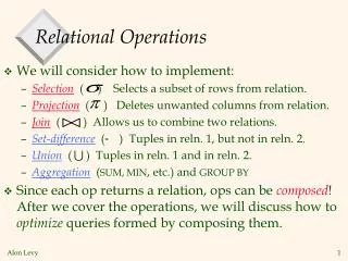
Relational Operations. We will consider how to implement: Selection ( ) Selects a subset of rows from relation. Projection ( ) Deletes unwanted columns from relation. Join ( ) Allows us to combine two relations.

E N D
Relational Operations • We will consider how to implement: • Selection ( ) Selects a subset of rows from relation. • Projection ( ) Deletes unwanted columns from relation. • Join ( ) Allows us to combine two relations. • Set-difference ( ) Tuples in reln. 1, but not in reln. 2. • Union( ) Tuples in reln. 1 and in reln. 2. • Aggregation (SUM, MIN, etc.) and GROUP BY • Since each op returns a relation, ops can be composed! After we cover the operations, we will discuss how to optimize queries formed by composing them.
Schema for Examples Sailors (sid: integer, sname: string, rating: integer, age: real) Reserves (sid: integer, bid: integer, day: dates, rname: string) • Reserves: • Each tuple is 40 bytes long, 100 tuples per page, 1000 pages. • Sailors: • Each tuple is 50 bytes long, 80 tuples per page, 500 pages.
SELECT * FROM Reserves R WHERE R.rname < ‘C%’ Simple Selections • Of the form • Size of result approximated as size of R * reduction factor; we will consider how to estimate reduction factors later. • With no index, unsorted: Must essentially scan the whole relation; cost is M (#pages in R). • With an index on selection attribute: Use index to find qualifying data entries, then retrieve corresponding data records. (Hash index useful only for equality selections.)
Using an Index for Selections • Cost depends on #qualifying tuples, and clustering. • Cost of finding qualifying data entries (typically small) plus cost of retrieving records (could be large w/o clustering). • In example, assuming uniform distribution of names, about 10% of tuples qualify (100 pages, 10000 tuples). With a clustered index, cost is little more than 100 I/Os; if unclustered, upto 10000 I/Os! • Important refinement for unclustered indexes: 1. Find qualifying data entries. 2. Sort the rid’s of the data records to be retrieved. 3. Fetch rids in order. This ensures that each data page is looked at just once (though # of such pages likely to be higher than with clustering).
General Selection Conditions • (day<8/9/94 AND rname=‘Paul’) OR bid=5 OR sid=3 • Such selection conditions are first converted to conjunctive normal form (CNF): (day<8/9/94 OR bid=5 OR sid=3 ) AND (rname=‘Paul’ OR bid=5 OR sid=3) • We only discuss the case with no ORs (a conjunction of terms of the form attr op value). • An index matches (a conjunction of) terms that involve only attributes in a prefix of the search key. • Index on <a, b, c> matches a=5 AND b= 3, but notb=3.
Two Approaches to General Selections • First approach:Find the most selective access path, retrieve tuples using it, and apply any remaining terms that don’t match the index: • Most selective access path: An index or file scan that we estimate will require the fewest page I/Os. • Terms that match this index reduce the number of tuples retrieved; other terms are used to discard some retrieved tuples, but do not affect number of tuples/pages fetched. • Consider day<8/9/94 AND bid=5 AND sid=3. A B+ tree index on day can be used; then, bid=5 and sid=3 must be checked for each retrieved tuple. Similarly, a hash index on <bid, sid> could be used; day<8/9/94 must then be checked.
Intersection of Rids • Second approach • Get sets of rids of data records using each matching index. • Then intersect these sets of rids • Retrieve the records and apply any remaining terms. • Consider day<8/9/94 AND bid=5 AND sid=3. If we have a B+ tree index on day and an index on sid, we can retrieve rids of records satisfying day<8/9/94 using the first, rids of recs satisfying sid=3 using the second, intersect, retrieve records and check bid=5.
SELECTDISTINCT R.sid, R.bid FROM Reserves R Implementing Projection • Two parts: (1) remove unwanted attributes, (2) remove duplicates from the result. • Refinements to duplicate removal: • If an index on a relation contains all wanted attributes, then we can do an index-only scan. • If the index contains a subset of the wanted attributes, you can remove duplicates locally.
Equality Joins With One Join Column SELECT * FROM Reserves R1, Sailors S1 WHERE R1.sid=S1.sid • In algebra: R S. Common! Must be carefully optimized. R S is large; so, R S followed by a selection is inefficient. • Assume: M tuples in R, pR tuples per page, N tuples in S, pS tuples per page. • In our examples, R is Reserves and S is Sailors. • We will consider more complex join conditions later. • Cost metric: # of I/Os. We will ignore output costs.
Simple Nested Loops Join foreach tuple r in R do foreach tuple s in S do if ri == sj then add <r, s> to result • For each tuple in the outer relation R, we scan the entire inner relation S. • Cost: M + pR * M * N = 1000 + 100*1000*500 I/Os. • Page-oriented Nested Loops join: For each page of R, get each page of S, and write out matching pairs of tuples <r, s>, where r is in R-page and S is in S-page. • Cost: M + M*N = 1000 + 1000*500 • If smaller relation (S) is outer, cost = 500 + 500*1000
Index Nested Loops Join foreach tuple r in R do foreach tuple s in S where ri == sj do add <r, s> to result • If there is an index on the join column of one relation (say S), can make it the inner and exploit the index. • Cost: M + ( (M*pR) * cost of finding matching S tuples) • For each R tuple, cost of probing S index is about 1.2 for hash index, 2-4 for B+ tree. Cost of then finding S tuples depends on clustering. • Clustered index: 1 I/O (typical), unclustered: upto 1 I/O per matching S tuple.
Examples of Index Nested Loops • Hash-index on sid of Sailors (as inner): • Scan Reserves: 1000 page I/Os, 100*1000 tuples. • For each Reserves tuple: 1.2 I/Os to get data entry in index, plus 1 I/O to get (the exactly one) matching Sailors tuple. Total: 220,000 I/Os. • Hash-index on sid of Reserves (as inner): • Scan Sailors: 500 page I/Os, 80*500 tuples. • For each Sailors tuple: 1.2 I/Os to find index page with data entries, plus cost of retrieving matching Reserves tuples. Assuming uniform distribution, 2.5 reservations per sailor (100,000 / 40,000). Cost of retrieving them is 1 or 2.5 I/Os depending on whether the index is clustered.
. . . Block Nested Loops Join • Use one page as an input buffer for scanning the inner S, one page as the output buffer, and use all remaining pages to hold ``block’’ of outer R. • For each matching tuple r in R-block, s in S-page, add <r, s> to result. Then read next R-block, scan S, etc. Join Result R & S Hash table for block of R (k < B-1 pages) . . . . . . Output buffer Input buffer for S
Sort-Merge Join (R S) i=j • Sort R and S on the join column, then scan them to do a ``merge’’ (on join col.), and output result tuples. • Advance scan of R until current R-tuple >= current S tuple, then advance scan of S until current S-tuple >= current R tuple; do this until current R tuple = current S tuple. • At this point, all R tuples with same value in Ri (current R group) and all S tuples with same value in Sj (current S group) match; output <r, s> for all pairs of such tuples. • Then resume scanning R and S. • R is scanned once; each S group is scanned once per matching R tuple.
Example of Sort-Merge Join • Cost: M log M + N log N + (M+N) • The cost of scanning, M+N, could be M*N (very unlikely!) • With 35, 100 or 300 buffer pages, both Reserves and Sailors can be sorted in 2 passes; total join cost: 7500. (BNL cost: 2500 to 15000 I/Os)
Refinement of Sort-Merge Join • We can combine the merging phases in the sorting of R and S with the merging required for the join. • With B > , where L is the size of the larger relation, using the sorting refinement that produces runs of length 2B in Pass 0, #runs of each relation is < B/2. • Allocate 1 page per run of each relation, and `merge’ while checking the join condition. • Cost: read+write each relation in Pass 0 + read each relation in (only) merging pass (+ writing of result tuples). • In example, cost goes down from 7500 to 4500 I/Os. • In practice, cost of sort-merge join, like the cost of external sorting, is linear.
Original Relation Partitions OUTPUT 1 1 2 INPUT 2 hash function h . . . B-1 B-1 B main memory buffers Disk Disk Partitions of R & S Join Result Hash table for partition Ri (k < B-1 pages) hash fn h2 h2 Output buffer Input buffer for Si B main memory buffers Disk Disk Hash-Join • Partition both relations using hash fn h: R tuples in partition i will only match S tuples in partition i. • Read in a partition of R, hash it using h2 (<> h!). Scan matching partition of S, search for matches.
Cost of Hash-Join • In partitioning phase, read+write both relns; 2(M+N). In matching phase, read both relns; M+N I/Os. • In our running example, this is a total of 4500 I/Os. • Sort-Merge Join vs. Hash Join: • Given a minimum amount of memory (what is this, for each?) both have a cost of 3(M+N) I/Os. Hash Join superior on this count if relation sizes differ greatly. Also, Hash Join shown to be highly parallelizable. • Sort-Merge less sensitive to data skew; result is sorted.