Download

1 / 70
700 likes | 812 Views
A Simpler Minimum Spanning Tree Verification Algorithm. Valerie King Algorithmica, 18:263–270, 1997. D94922004 陳冠宇 D96945017 林振慶 R96922013 黃于鳴 R96922028 廖鳳玉 R96922032 張瀠文 R96922035 曾照涵. 2008/05/22. Outline. Introduction Bor ů vka Tree Property

E N D
A Simpler Minimum Spanning Tree Verification Algorithm Valerie King Algorithmica, 18:263–270, 1997 D94922004 陳冠宇 D96945017 林振慶 R96922013 黃于鳴 R96922028 廖鳳玉 R96922032 張瀠文 R96922035 曾照涵 2008/05/22
Outline • Introduction • Borůvka Tree Property • Komlós’s Algorithm for a Full Branching Tree • Implementation • Data Structures • The Algorithm • More Details • Analysis • Conclusion and Open Problems
Outline • Introduction • Borůvka Tree Property • Komlós’s Algorithm for a Full Branching Tree • Implementation • Data Structures • The Algorithm • More Details • Analysis • Conclusion and Open Problems
University of Victoria. Research interests: Randomized algorithms and data structures. Applications to networks and computational biology. Distributed computing. Valerie King
Abstract • Problem: • Determine whether a given spanning tree in a graph is a minimal spanning tree. • In 1984, Komlós presented an algorithm: • A linear number of comparisons. • But nonlinear overhead to determine which comparisons to make. • This paper simplifies Komlós’s algorithm, and gives a linear time procedure using table lookup in the unit cost RAM model.
Related Works(1/2) • Tarjan (1979) • Path compression on balanced trees. • O(m α(m,n)), almost linear running time. • α(m,n) is a very slowly growing function. • O(m) storage space. • Komlós (1984) • O(m) binary comparisons between edge costs. • Non-linear time to determine which comparisons to make.
Related Works(2/2) • Dixon, Rauch, and Tarjan (1992) • O(m), linear time algorithm. • Combines Tarjan’s almost-linear-time algorithm and Komlós’s algorithm, with a preprocessing and table-look-up method for small subproblems. • Decompose the tree into a large subtree and many microtrees. • Path compression (Tarjan 1979) is used on the large subtree. • The comparison decision tree needed to implement Komlós’s strategy for each possible microtree is precomputed and stored in a table. Each microtree with its query paths is encoded. The table is used to loop up the appropriate comparisons to make. • Model of computation: binary comparison, addition, substraction on edge cost on unit-cost random-access machine.
Definitions(1/3) • A graphG = (V, E) with nnodes and medges. • A path of length k from x to y in G is a sequence of edges {x,v1},{v1,v2},…,{vk-1,y}. • A treeT = (V, E) is a graph such that T is connected and contains no cycles. • T is a spanning tree if a tree is a subgraph of G with the same vertex set as T.
Definitions(2/3) G = (V,EG) a graph with w(e) on its edges. T = (V,ET) is a spanning tree of G. T is a minimum spanning tree if is minimum among all spanning trees of G.
Definitions(3/3) • T(x,y): the set of edges in the path in a tree T from node x to nodey. • In a tree T, there is a unique path from x to y. • A rooted tree is a tree with a distinguished node called root. • A Full branching tree is a rooted tree with all leaves on the same level and each internal node having at least two children. • B(x,y): the set of edges in the path in a full branching tree B from leafx to leafy.
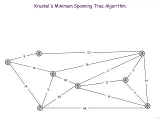
Key Observation(1/4) • A spanning tree is a minimum spanning tree iff the weight of each non-tree edge {u, v} is at least the weight of the heaviest edge in the path in the tree between u and v.
Key Observation(2/4) 4 3 a 2 1 4 2 5 1 x b 2 3 T(x,y) 1 2 1 y
Key Observation(3/4) 4 3 x a 2 1 4 5 1 y b 2 3 1 2 1
Key Observation(4/4) • These verification methods use this fact. • Find the heaviest edge in each such path for each non-tree edge {u,v} in the graph. • Compare the weight of {u,v} to it. 1 u 3 3 2 2 u v 3 3
Tree Path Problem • Finding the heaviest edges in the paths between specified pairs of nodes (“query paths”). 3 4 1 2 2
Main Ideas(1/2) • T is a spanning tree. • A simple O(n) algorithm to construct a full branching tree B with no more than 2n edges. • The weight of the heaviest edge in T(x, y) is the weight of the heaviest edge in B(x, y). • Use the version of the Komlós’s algorithm for full branching trees. • Much simpler than his algorithm for general trees.
Main Ideas(2/2) • Linear time implementation using table lookup of a few simple functions. • Can be constructed in time linear in the size of the tree. • Model of computation: unit random access model with word size θ(log n) bits. • Allow edge weights to be compared, added, or subtracted at unit cost.
Organization • The construction of full branching tree B • Proof of the property of B Komlós’s algorithm for determining the maximum weighted edge in each of m paths of a full branching tree • Implementation of Komlós’s algorithm: • Data structure • Algorithm • Details • Analysis
Outline • Introduction • Borůvka Tree Property • Komlós’s Algorithm for a Full Branching Tree • Implementation • Data Structures • The Algorithm • More Details • Analysis • Conclusion and Open Problems
Spanning TreeT Full Branching Tree B T B Full branching tree: rooted tree, leaves in same level, internal nodes have at least two children. • B has no more than 2n edges. • O(n) time to construct B. • The weight of the heaviest edge in T(x, y) is the weight of the heaviest edge in B(x, y).
Use Borůvka’s Algorithm(1/3) T • Tree B is constructed with node set W and edge set F by adding nodes and edges to B. • Initial phase: For each node v V, create a leaf f(v) of B. • B 1 2 3 6 4 7 8 5 9
Borůvka’s Algorithm (2/3) t1 t2 1 2 3 6 t4 3 4 4 9 3 9 4 7 8 5 9 Adding phase: Let A be the set of blue trees which are joined into one blue tree t in a phase i. Add a new node f(t) to W and add edge to F. T: B: t3 6 7 6
Borůvka’s Algorithm (3/3) 8 t t1 • Repeat edge contraction until there is one blue tree. • TB 10 8 11 8 11 10 t3 t4 t2 t4 t3 t1 t2 3 4 4 9 7 3 9 6 6 1 2 3 6 4 7 8 5 9 t
Borůvka’s Algorithm(3.001/3) t • Problem 1: Are edge weights in the path from leaf to root increased? • No,the weight of the edge which t1select may smaller than the edge weight in Tt1,for example: • But the weight of the edge which t1select must be bigger than the minimal edge weight in Tt1 4 4 B e T 4 5 a b d a d e c b Tt1 t1 t2 t1 t2 c 3 3 2 2 2 5 3
Borůvka’s Algorithm(3.002/3) • Problem 2: in adding phase, for each blue tree, if we choose the edge with the maximum weight, not minimal weight, does B still hold the property: • For any pair of nodes x and y in T, the weight of the heaviest edge in T(x, y) equals the weight of the heaviest edge in B(f(x), f(y)). • No,for example: • the weight of the heaviest edge in T(a, c) = 3, • the weight of the heaviest edge in B(a, c) = 5. 5 a b a b c T B c t1 3 3 5 5
The number of blue trees drops by a factor of at least two after each phase. B is a full branching tree. Theorem 1 For any pair of nodes x and y in T, the weight of the heaviest edge in T(x, y) equals the weight of the heaviest edge in B(f(x), f(y)). Borůvka’s Tree Property (1/5)
Claim1: for every edge , there is an edge such that w(e’)≥w(e). Then a = f(t) for some blue tree t which contains either x or y. Let e’ be the edge in T(x, y) with exactly one endpoint inblue tree t. Since t had the option of selecting e’,w(e’)≥w(e). Borůvka’s Tree Property (2/5) e e’’ r T B t b e Blue tree t Contains x f(y) e’ Blue tree t a f(t) f(x)
Claim2: Let e be a heaviest edge in T(x, y). Then there is an edge of the same weight in B(f(x), f(y)). e must be selected. Case1: If e is selected by a blue tree t which contains x or y, then an edge in B(f(x), f(y)) is labeled with w(e). Borůvka’s Tree Property (3/5) y r j T B i b e e t f(y) Blue tree t a f(t) Blue tree t contains x f(x)
Claim2: Let e be a heaviest edge in T(x, y). Then there is an edge of the same weight in B(f(x), f(y)). Case2: assume that e is selected by a blue tree i which does not contain x or y. This blue tree contained one endpoint of e and thus one intermediate node on the path from x to y. Therefore it is incident to at least two edges on the path. Then e is the heavier of two, giving a contradiction. Borůvka’s Tree Property (4/5) y r x T i B b e e j f(y) a f(i) Blue tree i
Claim1: for every edge , there is an edge such that w(e’)≥w(e). Claim2: Let e be a heaviest edge in T(x, y). Then there is an edge of the same weight in B(f(x), f(y)). Theorem: For any pair of nodes x and y in T, the weight of the heaviest edge in T(x, y) equals the weight of the heaviest edge in B(f(x), f(y)). Borůvka’s Tree Property (5/5)
Outline • Introduction • Borůvka Tree Property • Komlós’s Algorithm for a Full Branching Tree • Implementation • Data Structures • The Algorithm • More Details • Analysis • Conclusion and Open Problems
MST Verification UsingFull Branching Tree • Given a spanning tree T of a graph G. • Construct a full branching tree B from T using Borůvka’s algorithm. • For every non-tree edge e = {u, v} in G, find the heaviest edge e’ in the query path B(f(u), f(v)), and see if w(e) ≥w(e’) or not. • By Borůvka’s tree property. • If for all non-tree edge e, w(e) ≥w(e’), then T is a minimum spanning tree of G.
Komlós’s Algorithm (1/5) • Given a full branching tree with n nodes and m query paths between pairs of leaves, Komlós’s algorithm can compute the heaviest edge in every query path using only linear number of comparisons. • For each query path (leaf x -> leaf y), break up the path into two half-paths from leaf up to the lowest common ancestor of the pair. • Find the heaviest edge in each half-path and compare the two edges to determine the heaviest edge in the whole path.
Komlós’s Algorithm (2/5) • A(v): the set of all half paths of every query path which contain v restricted to the interval [root, v]. • Let p be the parent of v. A(v|p): the set of paths in A(v) restricted to the interval [root, p]. r query paths: a->d, c->e, b->f A(v) = {(v->p->s), (v->p)} A(v|p) = {(p->s)} A(p) = {(p->s), (p->s->r)} B s p v a e b f c d
Komlós’s Algorithm (3/5) • If we know the heaviest edge in each path in A(p), we can determine the heaviest edge in each path in A(v) through A(v|p). • Assume we know the heaviest edge in each path in A(p). • Because , we already know the heaviest edge in each path in A(v|p). • To determine the heaviest edge in each path in A(v), we need only to compare w(v, p) to the heaviest edge in each path in A(v|p). v p e1 e2 e3 e4
Komlós’s Algorithm (4/5) • Starting from the root, descend level by level and as each node v encountered, the heaviest edge in each path in A(v) can be determined. • For a query path(x->y), use A(x) and A(y) to determine the heaviest edge in each half path, and compare the two to determine the heaviest edge in the query path.
Komlós’s Algorithm (5/5) • The ordering of the weights of the heaviest edges in A(p) can be determined by the length of their respective paths, since for any two paths s and t in A(p), path s includes path t or vice versa. • Compare w(v, p) to each weight in A(v|p) can be done by using binary search. • Komlós shows that the upper bound on the number of comparisons needed to find the heaviest edge in each half path is v p e1 w(e4) ≥ w(e3) ≥ w(e2) ≥ w(e1) e2 e3 w(v, p) e4
Outline • Introduction • Borůvka Tree Property • Komlós’s Algorithm for a Full Branching Tree • Implementation • Data Structures • The Algorithm • More Details • Analysis • Conclusion and Open Problems
Node Label and Edge Tag 0000 0000 1000 0000 0010 0100 1000 0000 0001 0010 0011 0100 0101 0110 0111 1000 • Node Label - bits Leaves: the order of the results of DFS. Internal nodes: the longest all 0’s suffix in its subtree.
Node Label Property Example 2: • Nodes on the same level won’t possess the same label. Internal 0100 Example 1: Internal 0010 0110 … … … Leaf Leaf 0110 0111 0100 0010 0011 0010 0011 0110 0111
Node Label and Edge Tag 0000 < 1, 0 > < 1, 4 > 0000 1000 < 2, 0 > < 2, 2 > < 2, 3 > < 2, 4 > 2 0000 0010 0100 1000 < 3, 0 > < 3, 1 > < 3, 2 > < 3, 1 > < 3, 3 > < 3, 1 > < 3, 2 > < 3, 1 > < 3, 4 > 3 0000 0001 0010 0011 0100 0101 0110 0111 1000 • Edge tag - O( ) bits v : the endpoint which is farther from root. distance(v): v’s distance from root. i(v): index of the rightmost 1 in v’s label. < distance(v), i(v) >
LCA: Lowest Common Ancestor • LCA(v): • A vector with size • ith bit of LCA(v) = 1 iff there is a path in A(v) whose upper endpoint is at distance i from the root • For example: • Query paths: {(u, v), (u, w)} • A(u) = {(u, a), (u, r)} • LCA(u) = 1100 r a p u v w
BigLists and SmallLists (1/3) • If |A(v)| > wordsize / tagsize , |A(v)| is Big • Otherwise, |A(v)| is Small
BigLists and SmallLists (2/3) r BigList(u) <1, 0> (a, r) a <2, 0> (p, a) p • For example: • Query paths: {(u, v), (u, w)}. • A(u) = { (u, a), (u, r)}. • A1(u) = (a, r), A2(u) = (p, a). • |A(u)| = 2 > wordsize / tagsize = 4 / 4 = 1 • |A(u)| is big. u v w
BigLists and SmallLists (3/3) • For example: • Query path: {(c, d)}. • A(c) = {(c, b)}. • A1(c) =(c, b). • |A(c)| = 1 ≤ 1 • A(c) is small. SmallList(c) <3, 2> (c, b) b c d
Outline • Introduction • Borůvka Tree Property • Komlós’s Algorithm for a Full Branching Tree • Implementation • Data Structures • The Algorithm • More Details • Analysis • Conclusion and Open Problems
Goal of the Algorithm • Generate bigList(v) or smallList(v) in time proportional to log|A(v)|. • The time spent implementing Komlós’s algorithm at each node does not exceed the worst case number of comparisons needed at each node.
Implementation Details of the Algorithm (1/7) • The computation of the LCAs. • Compute all LCAs for each pair of endpoints of the m query paths. • Form the vector LCA(l) for each leaf l. • Form the vector LCA(v) for a node at distance i from the root by ORing together the LCAs of its children and setting the jth bits to 0 for all j≧i. • Compute all LCAs for each pair of endpoints of the m query paths using an algorithm that runs in time O(n + m).
Implementation Details of the Algorithm (2/7) 100 010 110 110 100 000 000 000 000 000 000 000 000 100 010
Implementation Details of the Algorithm (3/7) • Subword • tagsize bits: loglogn. • Swnum • The maximum number of subwords stored in a word.