Download
1 / 14
150 likes | 358 Views
Transformation & regression. Many seemingly nonlinear relationships can be linearized by data transformation. We cover four types of relationship Exponential growth or decay, y = y 0 e rt , or y= ab x with semi-log transformation

E N D
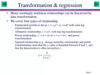
Transformation & regression • Many seemingly nonlinear relationships can be linearized by data transformation. • We cover four types of relationship • Exponential growth or decay, y = y0ert, or y=abxwith semi-log transformation • Allometric relationship, y = axb, with log-log transformation • Power relationship, y = a + bx or y = a + bx, and power transformation: • Sigmoid relationship (e.g., dosage-mortality relationship) and probit transformation (note that the y value is bounded between 0 and 1, and that the linearization is often not perfect.)
Growth curve of E. coli • A researcher wishes to estimate the growth curve of E. coli. He put a very small number of E. coli cells into a large flask with rich growth medium, and take samples every half an hour to estimate the density (n/L). • 14 data points over 7 hours were obtained. • What is the instantaneous rate of growth (r). What is the initial density (N0)? • As the flask is very large, he assumed that the growth should be exponential, i.e., y = a·ebt (Which parameter correspond to r and which to N0?)lny = lna + bt T Density 0.5 20.023 1 39.833 1.5 80.571 2 161.102 2.5 317.923 3 635.672 3.5 1284.544 4 2569.43 4.5 5082.654 5 10220.777 5.5 20673.873 6 40591.439 6.5 81374.642 7 163963.873
R functions md<-read.table("EcoliGrowth.txt",header=T) attach(md) plot(T,Density) lnD <- log(Density) fit<-lm(lnD~T) Alternatively, fit<-lm(log(Density)~T) summary(fit) anova(fit) plot(T,lnD) abline(fit) PredY<-exp(fitted(fit)) plot(T,Density) lines(T,PredY) nd<-data.frame(T=1.3) predict(fit,nd,interval="confidence") ci95<-predict(fit,md,interval="confidence") ci95Scaled<-exp(ci95) plot(T,Density) lines(T,ci95Scaled[,1],col="red") lines(T,ci95Scaled [,2],col="blue") lines(T,ci95Scaled [,3],col="blue") Run, and ask students to replace aand b in the equation y = a·ebtby estimated numbers. What is the initial density and the instantaneous growth rate? Does the output represent confidence limits of Density for T = 1.3?
Body weight of wild elephant • A researcher wishes to estimate the body weight of wild elephants. • He measured the body weight of 13 captured elephants of different sizes as well as a number of predictor variables, such as leg length, trunk length, etc. Through stepwise regression, he found that the inter-leg distance (shown in figiure) is the best predictor of body weight. • He learned from his former biology professor that the allometric law governing the body weight (W) and the length of a body part (L) states thatW = aLb • Use linear regression to find parameters a and b. L W 0.31 1.657 0.43 2.500 0.52 4.680 0.59 7.075 0.70 10.070 0.83 11.988 0.89 14.836 1.12 18.318 1.13 23.496 1.19 27.897 1.25 36.796 1.41 44.611 1.50 51.183
R functions md<-read.table("ElephantWt.txt",header=T) attach(md) plot(L,W) lnL <- log(L) lnW<- log(W) fit<-lm(lnW~lnL) summary(fit) anova(fit) plot(lnL,lnW) abline(fit) PredW<-exp(fitted(fit)) plot(L,W) lines(L,PredW) nd<-data.frame(lnL=log(1.3)) predict(fit,nd,interval="confidence") ci95<-predict(fit,md,interval="confidence") ci95Scaled<-exp(ci95) plot(L,W) lines(L,ci95Scaled[,1],col="red") lines(L,ci95Scaled [,2],col="blue") lines(L,ci95Scaled [,3],col="blue") Run, and ask students to replace aand b in the equation W = aLb by estimated numbers.
DNA and protein gel electrophoresis • How to estimate the molecular mass of a protein? • A ladder: proteins with known molecular mass • Deriving a calibration curve relating molecular mass (M) to migration distance (D): D = F(M) • Measure D and obtain M • The calibration curve is obtained by fitting a regression model
Protein molecular mass • The equation appears to describe the relationship between D and M quite well. This relationship is better than some published relationships, e.g., D = a – b ln(M) • The data are my measurement of D and M for a subset of secreted proteins from the gastric pathogen Helicobacter pylori (Bumann et al., 2002). • Assignment: Use data transformation and linear regression to obtain parameters a and b and a confidence plot as in Slide 7 (Report just the fitted equation and the plot in 1 page) Bumann, D., Aksu, S., Wendland, M., Janek, K., Zimny-Arndt, U., Sabarth, N., Meyer, T.F., and Jungblut, P.R., 2002, Proteome analysis of secreted proteins of the gastric pathogen Helicobacter pylori. Infect. Immun. 70: 3396-3403.
Area and Radius Assignment: Estimate area (A) by counting squares and partial squares within each circle, and radius (r) by the number of squares (and partial squares) from center to circumference. Use data transformation and linear regression to fit the relationship of A = arb (report only the fitted equation and confidence intervals of area given r = 3).
Power transformation x y 1 1.1882 4 1.2625 9 1.3506 17 1.4348 25 1.4897 33 1.5287 41 1.5602 49 1.5857 57 1.6105 65 1.6305 73 1.6497 81 1.6654 89 1.6816 97 1.6953 105 1.7094 113 1.7214 121 1.7335 129 1.7439 137 1.7554 Sometime we may encounter relationships such as y = a + bx and need to find the best to perform the transformation. Rational: the best is one that will yields the highest linear correlation between yand x. This approach is much more elegant than using the boxcox function in R
R functions md<-read.table("PowerTransform.txt",header=T) attach(md) plot(x,y) myF<-function(lambda) abs(cor(md$x,(md$y)^lambda)) sol<-optimize(myF,interval=c(1,20),maximum=T) lambda<-sol$maximum newY<-y^lambda plot(x,newY) fit<-lm(newY~x) CI95<-predict(fit,md,interval="confidence") CI95Scaled<-CI95^(1/lambda) plot(x,y) lines(x,CI95Scaled[,1],col="red") lines(x,CI95Scaled[,2],col="blue") lines(x,CI95Scaled[,3],col="blue")
Toxicity study: pesticide What transformation to use?
Probit and probit transformation • Probit has two names/definitions, both associated with standard normal distribution: • the inverse cumulative distribution function (CDF) • quantile function • CDF is denoted by (z), which is a continuous, monotone increasing sigmoid function in the range of (0,1), e.g.,(z) = p(-1.96) = 0.025 = 1 - (1.96) • The probit function gives the 'inverse' computation, formally denoted -1(p), i.e.,probit(p) = -1(p) probit(0.025) = -1.96 = -probit(0.975) • [probit(p)] = p, and probit[(z)] = z. 0.4 0.3 p 0.2 0.1 0.0 -3 -2 -1 0 1 2 3 z
R functions md<-read.table("Pesticide.txt",header=T) attach(md) plot(Dosage,Mortality) NuProbit<-qnorm(Mortality/100) fit<-lm(NuProbit~Dosage) summary(fit) anova(fit) plot(Dosage,NuProbit) abline(fit) PredM<-100*pnorm(fitted(fit)) plot(Dosage,Mortality) lines(Dosage,PredM) nd<-data.frame(Dosage=qnorm(31.3/100)) predict(fit,nd,interval="confidence") ci95<-predict(fit,md,interval="confidence") ci95Scaled<-100*pnorm(ci95) plot(Dosage,Mortality) lines(Dosage,ci95Scaled[,1],col="red") lines(Dosage,ci95Scaled [,2],col="blue") lines(Dosage,ci95Scaled [,3],col="blue") Why divide Percent by 100? Run and explain