Download
1 / 34
340 likes | 471 Views
ECE 590I. Line Limit Preserving Power System Equivalent. Wonhyeok Jang Work with Prof. Overbye , Saurav Mohapatra & Hao Zhu. Contents. Introduction Preliminaries Cases Algorithm Examples Conclusions. Introduction. Equivalent power system

E N D
ECE 590I Line Limit Preserving Power System Equivalent WonhyeokJang Work with Prof. Overbye, SauravMohapatra & Hao Zhu
Contents • Introduction • Preliminaries • Cases • Algorithm • Examples • Conclusions
Introduction • Equivalent power system • A model system with fewer nodes and branches than the original • Purpose of equivalent • More efficient simulation • Without sacrificing too much fidelity of simulation results of the original
Introduction • Ward equivalent (Kron’s reduction) • Traditional method to equivalence power system network models • Loses desired attributes of the original system • Objective of work • Develop equivalents that preserve desired attributes, the line limits in this work, of the original system
Preliminary – Line limits • Thermal line limits are intended to limit • Temperature attained by the energized conductors • Resulting sag • Loss of tensile strength • Limits are calculated where conductor sag is at minimum allowable clearance • Geographical condition • Climate condition
Preliminary - Kron’s reduction • When a bus k between bus i and j is equivalenced • First term on RHS is admittance of existing line • Second term on RHS is admittance of equivalent line • Theses equivalent lines have no limits • Goal is to assign limits to theses equivalent lines that preserve desired attribute of the original
Preliminary - PTDF • Power Transfer Distribution Factor • Linear approximation of the impact of power flowing on each line w.r.t the amount t of an arbitrary basic transaction w • ∆fl: fraction of power transfer flowing on line l • ∆t: specific amount of transaction w • Basic transaction
Preliminary - PTDF • PTDFs on the retained lines are not affected by equivalencing Original system with PTDFs from 2 to 3 Equivalent system with PTDFs from 2 to 3
Preliminary - MPT • Desired attribute to preserve by assigning limits • Maximum power transfer (MPT) between retained buses match that for the same buses in the original • MPT between bus i and j can be calculated with PTDF • l: each line of the system • Need to match for MPTs between all the first neighbor buses of the bus being eliminated
General Case • Bus E, between bus A and B, is going to be eliminated • Need to calculate the new limit for the equivalent line between bus A and B
Special Case • Series Combination • If two lines are in series and the node joining them is equivalenced, then the total limit must be the lower of the two limits
Special Case • Parallel Combination • New limit is determined by which line in the parallel lines is binding
Algorithm • Sequentially as each bus is being equivalenced • Combine limits of parallel lines • Calculate PTDFs between the first neighbor buses • Calculate MPT between the first neighbor buses, only considering the lines that are being eliminated • Limits on the retained lines do not need to be considered since they remain the same • Determine limits for equivalent lines so the MPTs of the equivalent match that in the original
Ex - 4 bus system • MPTs in the original system • MPT 2-3: 216.7 MW (1-3 binding) • MPT 2-4: 171.7 MW (1-4 binding) • MPT 3-4: 144.9 MW (1-4 binding) • For 2-3 direction, eq. line limits are • Lim23 >= 216.7*0.234 = 50.7 MW • Lim24 >= 216.7*0.024 = 5.2 MW • Lim34 >= 216.7*0.088 = 19.1 MW Original system with PTDF from 2 to 3 Reduced system with PTDF from 2 to 3
Ex - 4 bus system(Exact solution) • Often, solution is just the largest in each row • This works when each column has one solution • There are cases with no exact solutions when equality constraints for at least one direction may not by satisfied
Ex - 4 bus system(No solution 1 - Overestimate) • When there’s no solution -> Bound the solution • Line limit 1-4 is reduced from 60 MVA to 20 MVA • Others are all the same with the original • MPTs in the original system • MPT 2-3: 216.7 MW (1-3 binding) • MPT 2-4: 57.2 MW (1-4 binding) • MPT 3-4: 48.3 MW (1-4 binding) Original system with PTDF from 2 to 3
Ex - 4 bus system(No solution 1 - Overestimate) • All of the inequality constraints are satisfied for each row • But power flow in direction 3-4 is overestimated since no entries in its column is enforced
Ex - 4 bus system(No solution 2 - underestimate) • We make sure power flow in each direction is less than the original MPT • Then at least one inequality constraints would be violated and this will underestimate the MPT • We define “limit violation cost” for each entry of the matrix, which is the sum of violations for all entries in each row
Ex - 4 bus system(No solution 2 - underestimate) Original eq. line limit matrix • For the first row, the 2-3 entry is 0 since it involves no limit violations; • the 2-4 entry 57.4 = (50.7 – 1.6) + (9.9 – 1.6) • The 3-4 entry 40.8 = (50.7 – 9.9) Limit violation cost matrix
Ex - 4 bus system(No solution 2 - underestimate) • Minimum matching problem – Hungarian algorithm • Choose one entry in each row and each column that minimizes the sum of the violation costs Limit violation cost matrix Underestimate solution
Conclusions • Able to determine limits for eq. lines • In case of no exact limits, we bound the limits • When the number of first neighbor buses increase, then there’s rapid increase of the number of computation • There’s a certain value of line limits that turns a exact solution case to no exact solution case • Investigation of which factor changes solution types is needed
Ex - 7 bus system • Original 7-bus system • Eliminating bus 3
Ex - 7 bus system Determination of equivalent line limits MPT comparison of lines being eliminated between 7-bus and 6-bus MPT comparison of all lines between 7-bus and 6-bus
Ex - 7 bus system • Equivalent 6-bus system • Eliminating bus 5
Ex - 7 bus system Determination of equivalent line limits MPT comparison of lines being eliminated between 6-bus and 5-bus MPT comparison of all lines between 6-bus and 5-bus
Ex - 7 bus system • Equivalent 5-bus system • Eliminating bus 2
Ex - 7 bus system(overestimate) Determination of equivalent line limits
Ex - 7 bus system (overestimate) MPT comparison of lines being eliminated between 5-bus and 4-bus MPT comparison of all lines between 5-bus and 4-bus
Ex - 7 bus system (underestimate) Determination of equivalent line limits Limit violation costs
Ex - 7 bus system (underestimate) • Find minimum sum of limit violation costs using Hungarian algorithm
Ex - 7 bus system (underestimate) • Find minimum sum of limit violation costs using Hungarian algorithm
Ex - 7 bus system (underestimate) Determination of equivalent line limits
Ex - 7 bus system (underestimate) MPT comparison of lines being eliminated between 5-bus and 4-bus MPT comparison of all lines between 5-bus and 4-bus