Download
1 / 44
440 likes | 513 Views
Modeling sand transport and sandbar evolution along the Colorado River below Glen Canyon Dam. OUTLINE:. Available and unavailable data Kees’ model of the entire reach Our model of Eminence STEP 1: calibrating models hydrodynamically STEP 2: running morphodynamically

E N D
Modeling sand transport and sandbar evolution along the Colorado River below Glen Canyon Dam
OUTLINE: • Available and unavailable data • Kees’ model of the entire reach • Our model of Eminence • STEP 1: calibrating models hydrodynamically • STEP 2: running morphodynamically • Experiments adjusting sediment transport • STEP 3: Repeat for several types of models
Available data • Multibeam • Topo • Water-surface • ADCP velocity • Total station • HWM • Sediment Concentration • Bed D50 • Bar grain size Sediment Concentration Stage-Q Data Stage-Q Data Extent of HWM data
Unavailable data: • Topo in rapids • Stage-Q at likely model boundaries • Composition of bed sediment • Change in suspended concentration through reach Sediment Concentration Stage-Q Data Stage-Q Data Extent of HWM data
Available water-surface data: Multibeam sonar based water-surface elevations High-water marks surveyed post HFE
Longitudinal water-surface profiles: Eminence High-water marks are very noisy Only present info along the edge of river left Multibeam data provide spatial structure
Kees’ Model • 3D using 12 layers • Compressed hydrograph • Bed-evolution on • Roughness: Zo=0.01 m • 2D Turbulence: HLES on • 3D Turbulence: K-Epsilon • Incoming sediment concentration is 50% of measured • Thickness of sediment on bed is 1m everywhere
Kees’ 3D Model: Eminence Reach • Modeled ws is much lower than measured • Not able to match measured ws without: • Lowering the downstream boundary AND • Increasing the roughness significantly
Kees’ 3D Model: Eminence Reach • Thalweg shows a similar problem • BUT, water-surface is too high in lower eddy….. • Points to problems with topography in rapid between, boundary conditions and roughness
Eminence Models • 2D model and 3D (12 layers) • Compressed hydrograph • Roughness: variable • 2D Turbulence: HLES on • 3D Turbulence: K-Epsilon • Incoming sediment concentration is 100% of measured • Thickness of sediment on bed is based on min surface • Composition of bed sediment is based on D50 eyeball and σ from composited bar measurements
Eminence Model STEP 1: Calibrate the models hydraulically based on measured topo near end of peak (no bed evolution) STEP 2: Run model with bed evolution on with the HFE hydrograph and measured sediment
STEP 1: Calibration Strategy • Run model without bed evolution for topography at end of the peak using a range of possible z0 values • Using Ks=30* z0 for 2D model runs (White-Colebrook) • Compare to multibeam measured water surface points for same time period. • Compare ADCP velocity vectors and magnitude for similar time period. • Select z0 that provides the best hydraulic calibration
3D HLES: water surface • WS is reasonably well calibrated- although not very sensitive to zo • RMS=0.028 m
3D HLES: Water surface along thalweg Variable zo improves ws to a point, but increasing the upstream zo further doesn’t seem to change the ws much
3D HLES: Difference between modeled and measured water surface Z0=0.01 Z0=0.05 and 0.001 The variable roughness case seems to improve results in the eddy eye Z0=0.001 Z0=0.0001
3D HLES: vectors Eddy-eye is shifted upstream slightly
2D HLES: water surface • Modeled using similar range in zo (ks=30z0) • 3 sets of ks values give similar water-surface elevations
2D HLES: Difference between modeled and measured water surface T8 ks=0.03 and 1.5 (zo=0.001 and 0.05) RMS=0.043 T10 ks=0.003 and 1.5 (zo=0.0001 and 0.05) RMS=0.040 T11 ks=0.0003 and 1.5 (zo=0.00001 and 0.05) RMS=0.039 Extremely similar looking, very difficult to tell any difference based on ws. RMS for lower ks seems to be lower because the ws in the eddy-eye is lower. I don’t think RMS is reliable in this case…….
T8 ks=0.03 and 1.5 T10 ks=0.003 and 1.5 T11 ks=0.0003 and 1.5 2D with HLES: velocity vectors • Vectors are also essentially the same…… Minor changes in vectors…..
2D HLES: velocity Still only minor differences between all 3 roughness cases…..
STEP 1: Summary • 3D HLES: Looks reasonably well calibrated based on: • WS elevations look quite good • Velocity magnitude looks good • Velocity vectors are on the right track • 2D HLES: Not clear which z0 combination is best—probably fine to use similar values to the 3D case.
STEP 2: Morphodynamics • Once models are hydrodynamically calibrated, run with bed evolution using: • Pre-HFL topography • Measured suspended sediment concentration • Measured thickness of bed material • Estimated composition of bed material • Based on average D50 from Eyeball assuming log-normal distributions with =1.6 estimated from composited samples from the Eminence bar
STEP 2: 3D HLES Morphodynamics Measured change: Modeled change: • Bar extends too far upstream and is too high • Significant deposition in eddy eye, rather than the measured scour • Return channel is not strongly defined • Large bar develops on river right just above the downstream rapid. This occurs where velocity is lower than measured (no eddy develops in the model) • Too much scour through the thalweg
STEP 2: 3D HLES Morphodynamics Measured change: Modeled change (Liz): See similar trends in model from Liz, although her model develops a stronger return channel, deposits more sediment in the eye and less on the rest of the bar. Liz’s model uses similar thickness and bed composition, but 50% the suspended sand concentration and different sediment transport relation.
STEP 2: 2D HLES Morphodynamics Measured change: Modeled change (ks=0.001 and 1.5): Modeled change (ks=0.0001 and 1.5): Modeled change (ks=0.00001 and 1.5):
Pre-peak Topo Post-peak Topo 3DHLES (z0=0.001 and 0.05) 2DHLES (ks=0.03 and 1.5) 2DHLES (ks=0.003 and 1.5) 2DHLES (ks=0.0003 and 1.5) STEP 2: Cross-sections 2D models build bars further into the main channel 3D model builds a reasonable bar, but scours bed
Pre-peak Topo Post-peak Topo 3DHLES (z0=0.001 and 0.05) 2DHLES (ks=0.03 and 1.5) 2DHLES (ks=0.003 and 1.5) 2DHLES (ks=0.0003 and 1.5) STEP 2: Cross-sections Both models build a bar in the eddy eye rather than scouring 2D models also appear to deposit sediment in the thalweg
Pre-peak Topo Post-peak Topo 3DHLES (z0=0.001 and 0.05) 2DHLES (ks=0.03 and 1.5) 2DHLES (ks=0.003 and 1.5) 2DHLES (ks=0.0003 and 1.5) STEP 2: Cross-sections Both models build a higher elevation bar further in the main channel than measured 2D models also appear to deposit sediment in the thalweg
Pre-peak Topo Post-peak Topo 3DHLES (z0=0.001 and 0.05) 2DHLES (ks=0.03 and 1.5) 2DHLES (ks=0.003 and 1.5) 2DHLES (ks=0.0003 and 1.5) STEP 2: Cross-sections Both models build the river right bar too far into the main channel 2D models deposits material in the thalweg, 3D model erodes.
Pre-peak Topo Post-peak Topo 3DHLES (z0=0.001 and 0.05) 2DHLES (ks=0.03 and 1.5) 2DHLES (ks=0.003 and 1.5) 2DHLES (ks=0.0003 and 1.5) STEP 2: Cross-sections 3D and 2D models over build bars on channel margins and scour the bed 2D models build a larger river left bar
STEP 2: Summary • 2D and 3D models over build the bars in terms of elevation and spatial extent into the main channel. • 3D HLES appears somewhat better than 2D HLES • 2D HLES build bars further into the channel • 2D HLES deposits material in the thalweg, rather than scouring • Model Time comparisons: • 3D HLES model runs take 1+ hrs • 2D HLES model runs take ~2-3 minutes
What can improve bed evolution prediction? • 3D HLES bed evolution needs improvement: • Use van Rijn 1984? • Adjust van Rijn roughness height? • Adjust bed composition? • Avalanching processes? • Change diffusivity? • Other ideas?
Morphodynamics for several transport cases Measured change: Modeled change: T40 (zo=0.001 and 0.05) Modeled change: T40 Rh=2 Modeled change: T40 coarser bed Modeled change: T40 vr84 Liz Modeled change: T40 vr84 Kees Modeled change: T40 Diffusivity=0.0001
Pre-peak Topo Post-peak Topo 3DHLES (z0=0.001 and 0.05) 3DHLES (z0=0.001 and 0.05)- coarser bed composition 3DHLES (z0=0.001 and 0.05)- Van Rijn 1984—Kees ws 3DHLES (z0=0.001 and 0.05)- Van Rijn 1984—Liz 3DHLES (z0=0.001 and 0.05)- Rh=2, not 1 3DHLES (z0=0.001 and 0.05)- HED=0.0001, not 0.5 Morphodynamics for several cases All fairly similar, except the van Rijn 1984 model with Kees’ low settling velocities. This model builds lower bars, but fills in the thalweg……
Pre-peak Topo Post-peak Topo 3DHLES (z0=0.001 and 0.05) 3DHLES (z0=0.001 and 0.05)- coarser bed composition 3DHLES (z0=0.001 and 0.05)- Van Rijn 1984—Kees ws 3DHLES (z0=0.001 and 0.05)- Van Rijn 1984—Liz 3DHLES (z0=0.001 and 0.05)- Rh=2, not 1 3DHLES (z0=0.001 and 0.05)- HED=0.0001, not 0.5 Morphodynamics for several cases
Summary effects for different transport cases: • van Rijn 1984 vs 2000 • changing transport relation can produce large changes in the bed depending on how it is parameterized…..needs more work • Adjust roughness height • See marginal changes • Adjust bed composition • Bed evolution appears insensitive to bed composition (actually a plus since we don’t have detailed information about bed composition) • Adjusting Horizontal eddy diffusivity • Did not see substantial change in morphology…needs more work • Avalanching processes • Could prevent the bars from developing too far into the main channel. Need help from Kees to employ • Other ideas?
Morphodynamics for two sediment conditions Modeled change: 3DHLES- no suspended sediment at input, measured sediment thickness on bed Modeled change: 3DHLES- measured suspended sediment at input, 10 cm sediment bed thickness Measured change: Looks like the majority of the sediment deposited in the bar comes from the suspended sediment, rather than from material available on the bed in the reach
Pre-peak Topo Post-peak Topo 3DHLES (z0=0.001 and 0.05) 2DHLES (ks=0.03 and 1.5) 3DHLES (z0=0.001 and 0.05)- no input suspended sed 3DHLES (z0=0.001 and 0.05)- 10 cm thick bed Morphodynamics for two sediment conditions No input suspended sediment reduces deposition of sediment in eddy eye and scours bed 2 cm of sediment on the bed and the full suspended load changes the results very little.
Pre-peak Topo Post-peak Topo 3DHLES (z0=0.001 and 0.05) 2DHLES (ks=0.03 and 1.5) 3DHLES (z0=0.001 and 0.05)- no input suspended sed 3DHLES (z0=0.001 and 0.05)- 10 cm thick bed Morphodynamics for two sediment conditions No input suspended sediment may erode the bar in some places……. 2 cm of sediment on the bed and the full suspended load reduces height of bar somewhat
Pre-peak Topo Post-peak Topo 3DHLES (z0=0.001 and 0.05) 2DHLES (ks=0.03 and 1.5) 3DHLES (z0=0.001 and 0.05)- no input suspended sed 3DHLES (z0=0.001 and 0.05)- 10 cm thick bed Morphodynamics for two sediment conditions No input suspended sediment at the input erodes the channel significantly 2 cm of sediment on the bed and the full suspended load looks quite similar to the 2D results, but the bed is prevented from eroding……
STEP 3: Apply 1 and 2 to other models • Calibrate hydrodynamic calibration for: • 3D model with HLES—Complete • 3D model without HLES—in progress • 2D model with HLES—Complete • 2D model without HLES—in progress • 2D model with Secondary—in progress
Comparisons: • Velocity vectors • (compared to measured at end of peak 3/8/08_15:00) • Velocity magnitude • (compared to measured at end of peak 3/8/08_15:00) • Topography • (compared to measured after peak 3/10/08) • Cumulative erosion/deposition • Binned erosion/deposition by elevation • Select cross-sections • Model efficiency • Run time
Ideal info for modeling other sites: • Stage-Q relationship at downstream end of reach • Water-surface profiles at flows of interest • Topography- need detailed topo entire area of interest. • Select reaches with good entrance and exit conditions • Hydrograph • Suspended sediment concentration for hydrograph • Estimate of bed thickness (minimum surface maps) • Estimate of bed grain size distribution (Average D50 from eyeball/ from bar grain size analysis)