Download
1 / 30
300 likes | 457 Views
Mercury’s Seasonal Na Exosphere Data from MESSENGER’s MASCS UVVS instrument. Tim Cassidy, Aimee Merkel, Bill McClintock, Matt Burger Menelaos Sarantos , Rosemary Killen, Ron Vervack , Ann Sprague. Just how bright is the Na exosphere?.

E N D
Mercury’s Seasonal Na Exosphere Data from MESSENGER’s MASCS UVVS instrument Tim Cassidy, Aimee Merkel, Bill McClintock, Matt Burger MenelaosSarantos, Rosemary Killen, Ron Vervack, Ann Sprague
Just how bright is the Na exosphere? We see the Na exosphere because Na scatters sunlight ~589 nm (yellow) Potter et.al. (2001) From http://www.ips.gov.au/Category/Educational/Space%20Weather/The%20Aurora/Aurora.pdf
Messenger UVVS data is especially valuable because it gives high resolution vertical profiles (‘limb scans’) of the atmosphere Killen et al., 2008 vs. Potter and Morgan, 1990 Earth-based Na observations Messenger limb scan
For Na, we will focus on near-surface (<1000 km) limb scans What is a limb scan and why is it useful? column density or radiance lines of sight hot cold Altitude Of particular interest is the slope of the limb scan—which tells us the energy of ejected Na Gravity acts as an energy spectrometer.
This talk is about the dayside, which is typically probed near the equator: Note: poles are harder to investigate with MESSENGER’s orbit. MESSENGER also has a lot of tail data, not presented here.
To get atmospheric properties we have fitted limb scans with a simple function, called a Chamberlain model. Chamberlain model: density ~ n0e-U/kT where U is the potential energy (times another factor called zeta…) sunlight Gravitational potential Radiation acceleration term, analogous to U = -mgh Note: Radiation acceleration is up to ½ Mercury’s gravity Chamberlain model fits give us two parameters: surface density and temperature
Need to account for line of sight: line of sight column density = Integral of density over line of sight≈ surface density*2*K*H where K~Sqrt(pi*r/2H) H = kT/mg where g is the sum of gravitational and radial photon acceleration lines of sight
Example limb scan fits: I am going to focus on the dense lower exosphere in this talk What is it’s temperature? What is its density? How does it vary? And what do these tell us about the process that launches molecules off the the surface?
Results, part I: Na temperature TAA Temperature is roughly constant 180° 0° Example: temperature at noon local time Data from over 6 Mercury years This excludes the high temperature ‘tail’ at high altitudes mentioned earlier. Modelers predicted a more variable temperature…
And temperature is the same across dayside: (some data points randomly excluded for clarity)
Compared with ground-based observations of the temperature: 700-1500 K 2008 Killen et al., 1999: 1500 K (at equator)
We can compare with possible ejection mechanisms • Thermal Desorption • <700 K • (and thermal accommodation) • PSD • Photon Stimulated Desorption • similar to ESD, electron stimulated • desorption • Meteorite Impact Vaporization • 1000s degrees • Sputtering • thousands to 10s of thousands • of degrees • Molecular dissociation • (e.g. CaXCa + X + energy) • 10s of thousands of degrees Experimental Data (Yakshinskiy and Madey, 1999 & 2004) 900 K Maxwellian PSD from ice Johnson et al., (2002) Conclusion: PSD is the best match to supply the near-surface exosphere temperature The temperatures we derive are similar to, but slightly colder, than Earth-based observations (Killen et al., 2008) There is no evidence of thermal desorption
But PSD would quickly deplete surface of Na, Na must be continually resupplied to surface by other processes such as impacts or ion-enhanced diffusion (e.g., Killen et al., 2008).
Plotting vs true anomaly angle shows pattern: (for this example, we use limbscans at 10:00 local time) TAA 180° 0° Data from over 6 Mercury years Perihelion Perihelion Aphelion
Different local times have similar (but distinct) patterns (some data points randomly excluded for clarity)
TAA 180° 0° Suggests correlation with radiation acceleration, as some ground based observations suggest Potter et al., 2009
TAA 180° 0° Compared with ground-based data (Potter et al 2007) Lines show model of Smyth and Marconi (2005) It’s difficult to compare with ground based data, which tends to report disk-averaged quantities. A large effort would be required to do this.
But perhaps the closest model: TAA 180° 0° Exosphere content from ‘PSD enhanced’ modeling scenario Leblanc and Johnson, 2010
Conclusions about Dayside Na • Strong evidence that PSD supplies lower dayside atmosphere • -temperature (~1200K) • -variation in noon density with TAA like Leblanc predicted in his ‘enhanced PSD’ simulation • -no evidence of thermal accommodation/thermal desorption • These trends are consistent • These limb scan column densities • don’t change much from year to year: • 20% standard deviation E.g., Noon, TAA 150-170° • There is no detailed comparison with models. • Ground-based data does not seem to match our results. Observation geometry? • Na has abundance comparable to O.
Compared to atomic oxygen Estimate of O vertical column density: If O is hot (10's of thousands of degrees), then the vertical column density is of the same order as the line-of-sight density near the surface, which can found from the observed O emissions, about 4 Rayleighs, and the O g value (~1E-4/sec, Killen et al., 2009): =4 Rayleighs/g value*1E6 (/cm2) = 4E10 cm-2 (regardless of the O temperature, this is an upper limit) vs Na:
Compared to Other Species • Ca • Ejected mostly from dawn and density peaks near perihelion—impact vaporization? • High temperature (15,000-25,000 K): molecular dissociation of impact vapor • Mg • Uncertain mix of temperatures • Nightside source needed Na Mg Ca Observed column densities: Na has a two components, two temperatures. It dominates near surface. Mg and Ca have single temperature. Mg dominates further from the surface.
Others suggested that same correlation Others did not: Killen et al. (2008)
Test: comparison of Chamberlain model with Matt’s Monte Carlo model, the gold standard --- Chamberlain with photon pressure 3000 K 1500 K 900 K Chamberlain model overestimates densities near dawn and dusk, where the Chamberlain model assumes no photon pressure effects (cos(chi)~0 in previous slide).