Download
1 / 32
320 likes | 483 Views
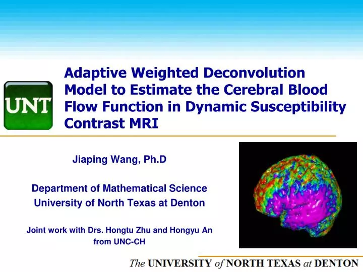
Adaptive Weighted Deconvolution Model to Estimate the Cerebral Blood Flow Function in Dynamic Susceptibility Contrast MRI. Jiaping Wang, Ph.D Department of Mathematical Science University of North Texas at Denton Joint work with Drs. Hongtu Zhu and Hongyu An f rom UNC-CH. Outline.

E N D
Adaptive WeightedDeconvolutionModel to Estimate the Cerebral Blood Flow Function in Dynamic Susceptibility Contrast MRI Jiaping Wang, Ph.D Department of Mathematical Science University of North Texas at Denton Joint work with Drs. Hongtu Zhu and Hongyu An from UNC-CH
Outline Background and Motivation Adaptive Weighted De-convolution Model Simulation Studies Real Data Analysis
Background Dynamic Susceptibility Contrast (DSC) Perfusion MRImeasures the passage of a bolus of a non-diffusible contrast through the brain. The signal decreases as the bolus passes through the imaging slices.
Convolution Relationship = R(t) where Ca(t) is the given AIF, C(t) is the observed concentration function, which is computed as S(t)/S0. We are interested in estimating the residue function R(t).
Deconvolution Techniques SVD Fourier Transformation TSVD at 0.01 TSVD at 0.1 TSVD at 0.05 TSVD at 0.2
Notations D : 3D volume N: the number of points on D d : a voxel in D : : spatial-temporal process : error process : AIF function, constant along space : Residue function
Voxel-wise Approach • Temporal-Domain • Frequency-Domain
Continuous Discrete Key Assumptions:
Voxel-wise vs. Spatio-Interdependence Jumping Space Irregular Boundary Two Main Steps (Spatial Adaptive Approach): 1. Transform the time series into the Fourier or Wavelet domain. 2. Smoothing the curves in the frequency domain by involving the local neighborhood information.
Spatial-Adaptive Approach Unknown Approximation
Weighted LSE Estimated HRF
Being Hierarchical Drawing nested spheres with increasing radiuses at each voxel and each frequency …
Being Adaptive • Sequentially determine weights • Adaptively update Stopping Statistics
Simulation Set-up (iv) (i) (ii) (iii) (i) A temporal cut of the true images; (iii) The true curves R(t) (ii) The true curves C(t) (iv) The AIF Curve The true residue curves
Simulation Results Result from SWADM Mean Curves of Clusters from SWADM Cluster Result Comparison Statistics: Dd= Where Xd is the estimated curve from the proposed method, Yd is from other methods including voxel-wise inverse Fourier Transformation (IFT), SVD, TSVD at thresholds 0.01, 0.05, 0.1 and 0.2, respectively. ||•|| is a norm operator.
Comparison Results (1) Comparison with SVD; (3) Comparison with TSVD at 0.05; (2) Comparison with TSVD at 0.01; (4) Comparison with TSVD at 0.1; (6) Comparison with Voxel-wise IFT; (5) Comparison with TSVD at 0.2;
Comparison along SNRs SVD TSVD at 0.01 TSVD at 0.05 TSVD at 0.1 TSVD at 0.2 Voxel-wise IFT Average of Dd along different SNRs One sample t test for Dd
Data Description The DSC PWI data set obtained from an acute ischemic stroke patient at Washington University in St. Louis after receiving a signed consent form with Institutional Review Board approval. MR images were acquired on a 3T Siemens whole body Trio system (Siemens Medical Systems, Erlangen, Germany). PWI images were acquired with a T2*-weighted gradient echo EPI sequence (TR/TE= 1500/43 ms,14 slices with a slice thickness of 5 mm, matrix= 128x128). This sequence was repeated 50 times and Gadolinium diethylenetriaminepenta-acetic acid (Gd-DTPA, 0.1 mmol/kg) was injected at the completion of the 5th measure. (e)
Clustering Results Sample of C(t) curves, the largest one can be considered as AIF. Slices from C(t) images Mean curves of clusters Clustered pattern
Estimation Results from Different Methods The curves from same voxel in Cluster I The curves from same voxel in Cluster II