Download
1 / 57
570 likes | 781 Views
MPI User-defined Datatypes. Techniques for describing non-contiguous and heterogeneous data. Derived Datatypes. Communication mechanisms studied to this point allow send/recv of a contiguous buffer of identical elements of predefined datatypes.

E N D
MPI User-defined Datatypes Techniques for describing non-contiguous and heterogeneous data
Derived Datatypes • Communication mechanisms studied to this point allow send/recv of a contiguous buffer of identical elements of predefined datatypes. • Often want to send non-homogenous elements (structure) or chunks that are not contiguous in memory • MPI allows derived datatypes for this purpose.
MPI type-definition functions • MPI_Type_Contiguous: a replication of datataype into contiguous locations • MPI_Type_vector: replication of datatype into locations that consist of equally spaced blocks • MPI_Type_create_hvector: like vector, but successive blocks are not multiple of base type extent • MPI_Type_indexed: non-contiguous data layout where displacements between successive blocks need not be equal • MPI_Type_create_struct: most general – each block may consist of replications of different datatypes • Note: the inconsistent naming convention is unfortunate but carries no deeper meaning. It is a compatibility issue between old and new version of MPI.
MPI_Type_contiguous • MPI_Type_contiguous (int count, MPI_Datatype oldtype, MPI_Datatype *newtype) • IN count (replication count) • IN oldtype (base data type) • OUT newtype (handle to new data type) • Creates a new type which is simply a replication of oldtype into contiguous locations
MPI_Type_contiguous example /* create a type which describes a line of ghost cells */ /* buf[1..nxl] set to ghost cells */ int nxl; MPI_Datatype ghosts; MPI_Type_contiguous (nxl, MPI_DOUBLE, &ghosts); MPI_Type_commit(&ghosts) MPI_Send (buf, 1, ghosts, dest, tag, MPI_COMM_WORLD); .. .. MPI_Type_free(&ghosts);
Typemaps • Each MPI derived type can be described with a simple Typemap, which specifies • a sequence of primitive types • A sequence of integer displacements Typemap = {(type0, disp0), …,(typen-1, dispn-1)} • i’th entry has type typei and displacement buf + dispi • Typemap need not be in any particular order • A handle to a derived type can appear in a send or recv operation instead of a predefined data type (includes collectives)
Question • What is typemap of MPI_INT, MPI_DOUBLE, etc.? • {(int,0)} • {(double, 0)} • Etc.
Typemaps, cont. • Additional definitions • lower_bound(Typemap) = min dispj , j = 0, …, n-1 • upper_bound(Typemap) = max(dispj + sizeof(typej)) + e • extent(Typemap) =upper_bound(Typemap) - lower_bound(Typemap) • If typei requires alignment to byte address that is a multiple of ki then e is least increment to round extent to next multiple of max ki
Question • Assume that Type = {(double, 0), (char, 8)} where doubles have to be strictly aligned at addresses that are multiples of 8. What is the extent of this datatype? ans: 16 • What is extent of type {(char, 0), (double, 8)}? ans: 16 Is this a valid type: {(double, 8), (char, 0)}? ans: yes, order does not matter
Detour: Type-related functions • MPI_Type_get_extent (MPI_Datatype datatype, MPI_Aint *lb, MPI_Aint *extent) • IN datatype (datatype you are querying) • OUT lb (lower bound of datatype) • OUT extent (extent of datatype) • Returns the lower bound and extent of datatype. • Question: what is upper bound? • lower_bound + extent
MPI_Type_size • MPI_Type_size(MPI_Datatype datatype, int *size) • IN datatype (datatype) • OUT size (datatype size) • Returns number of bytes actually occupied by datatype, excluding strided areas. • Question: what is size of {(char,0), (double, 8)}?
MPI_Type_vector • MPI_Type_vector(int count, int blocklength, int stride, MPI_Datatype oldtype, MPI_Datatype *newtype); • IN count (number of blocks) • IN blocklength (number of elements per block) • IN stride (spacing between start of each block, measured in # elements) • IN oldtype (base datatype) • OUT newtype (handle to new type) • Allows replication of old type into locations of equally spaced blocks. Each block consists of same number of copies of oldtype with a stride that is multiple of extent of old type.
MPI_Type_vector, cont • Example: Imagine you have an local 2d array of interior size mxn with ngghostcells at each edge. If you wish to send the interior (non ghostcell) portion of the array, how would you describe the datatype to do this in a single MPI call? • Ans: MPI_Type_vector (n, m, m+2*ng, MPI_DOUBLE, &interior); MPI_Type_commit (&interior); MPI_Send (f, 1, interior, dest, tag, MPI_COMM_WORLD)
Typemap view • Start with Typemap = {(double, 0), (char, 8)} • What is Typemap of newtype? MPI_Type_vector(2,3,4,oldtype,&newtype) Ans: {(double, 0), (char, 8),(double,16),(char,24),(double,32),(char,40), (double,64),(char,72),(double,80),(char,88),(double,96),(char,104)}
Question • Express MPI_Type_contiguous(count, old, &new); as a call to MPI_Type_vector. • Ans: • MPI_Type_vector (count, 1, 1, old, &new) • MPI_Type_vector (1, count, num, old, &new)
MPI_Type_create_hvector • MPI_Type_create_hvector (int count, int blocklength, MPI_Aint stride, MPI_Datatype old, MPI_Datatype *new) • IN count (number of blocks) • IN blocklength (number of elements/block) • IN stride (number of bytes between start of each block) • IN old (old datatype) • OUT new (new datatype) • Same as MPI_Type_vector, except that stride is given in bytes rather than in elements (‘h’ stands for ‘heterogeneous).
What is the MPI_Type_create_hvector equivalent of MPI_Type_vector (2,3,4,old,&new), with Typemap={(double,0),(char,8)}? Answer MPI_Type_create_hvector(2,3,4*16,old,&new) Question
Question For the following oldtype: Sketch the newtype created by a call to: MPI_Type_create_hvector(3,2,7,old,&new) Answer:
Example 1 – sending checkered region Use MPI_type_vector and MPI_Type_create_hvector together to send the shaded segments of the following memory layout:
Example, cont. double a[6][5], e[3][3]; MPI_Datatype oneslice, twoslice MPI_Aint lb, sz_dbl int mype, ierr MPI_Comm_rank (MPI_COMM_WORLD, &mype); MPI_Type_get_extent (MPI_DOUBLE, &lb, &sz_dbl); MPI_Type_vector (3,1,2,MPI_DOUBLE, &oneslice); MPI_Type_create_hvector (3,1,10*sz_dbl, oneslice, &twoslice); MPI_Type_commit (&twoslice);
Example 2 – matrix transpose double a[100][100], b[100][100] int mype MPI_Status *status; MPI_Aint row, xpose, lb, sz_dbl MPI_Comm_rank (MPI_COMM_WORLD, &mype); MPI_Type_get_extent (MPI_DOUBLE, &lb, &sz_dbl); MPI_Type_vector (100, 1, 100, MPI_DOUBLE, &row); MPI_Type_create_hvector (100, 1, 100*sz_dbl, row, &xpose); MPI_Type_commit (&xpose); MPI_Sendrecv (&a[0][0], 1, xpose, mype, 0, &b[0][0], 100*100, MPI_DOUBLE, mype, 0, MPI_COMM_WORLD, &status);
Example 3 -- particles Given the following datatype: Struct Partstruct{ char class; /* particle class */ double d[6]; /* particle x,y,z,u,v,w */ char b[7]; /* some extra info */ }; We want to send just the locations (x,y,z) in a single message. Struct Partstruc particle[1000]; int dest, tag; MPI_Datatype locationType; MPI_Type_create_hvector (1000, 3, sizeof(struct Partstruct), MPI_DOUBLE, &locationType);
MPI_Type_indexed • MPI_Type_indexed (int count, int *array_of_blocklengths, int *array_of_displacements, MPI_Datatype oldtype, MPI_Datatype *newtype); • IN count (number of blocks) • IN array_of_blocklengths (number of elements/block) • IN array_of_displacements (displacement for each block, measured as number of elements) • IN oldtype • OUT newtype • Displacements between successive blocks need not be equal. This allows gathering of arbitrary entries from an array and sending them in a single message.
Example Given the following oldtype: Sketch the newtype defined by a call to MPI_Type_indexed with: count = 3, blocklength = [2,3,1], displacement = [0,3,8] Answer:
Example: upper triangular transfer Consecutive memory
Upper-triangular transfer double a[100][100]; Int disp[100], blocklen[100], i, dest, tag; MPI_Datatype upper; /* compute start and size of each row */ for (i = 0; i < 100; ++i){ disp[i] = 100*i + i; blocklen[i] = 100 – i; } MPI_Type_indexed(100, blocklen, disp, MPI_DOUBLE, &upper); MPI_Type_commit(&upper); MPI_Send(a, 1, upper, dest, tag, MPI_COMM_WORLD);
MPI_Type_create_struct • MPI_Type_create_struct (int count, int *array_of_blocklengths, MPI_Aint *array_of_displacements, MPI_Datatype *array_of_types, MPI_Datatype *newtype); • IN count (number of blocks) • IN array_of_blocklengths (number of elements in each block) • IN array_of_displacements (byte displacement of each block) • IN array_of_types (type of elements in each block) • OUT newtype • Most general type constructor. Further generalizes MPI_Type_create_indexed in that it allows each block to consist of replications of different datatypes. The intent is to allow descriptions of arrays of structures as a single datatype.
Example Given the following oldtype: Sketch the newtype created by a call to MPI_Type_create_struct with the count = 3, blocklength = [2,3,4], displacement = [0,7,16] Answer:
Example Struct Partstruct{ char class; double d[6]; char b[7]; } Struct Partstruct particle[1000]; Int dest, tag; MP_Comm comm; MPI_Datatype particletype; MPI_Datatype type[3] = {MPI_CHAR, MPI_DOUBLE, MPI_CHAR}; int blocklen[3] = {1, 6, 7}; MPI_Aint disp[3] = {0, sizeof(double), 7*sizeof(double)}; MPI_Type_create_struct(3, blocklen, disp, type, &Particletype); MPI_Type_commit(&Particletype); MPI_Send(particle, 1000, Particletype, dest, tag, comm);
Alignment • Note, this example assumes that a double is double-word aligned. If double’s are single-word aligned, then disp would be initialized as (0, sizeof(int), sizeof(int) + 6*sizeof(double)) • MPI_Get_address allows us to write more generally correct code.
MPI_Type_commit • Every datatype constructor returns an uncommited datatype. Think of commit process as a compilation of datatype description into efficient internal form. • Must call MPI_Type_commit(&datatype). • Once commited, a datatype can be repeatedly reused. • If called more than once, subsequence call has no effect.
MPI_Type_free • Call to MPI_Type_free (&datatype) sets the value of datatype to MPI_DATATYPE_NULL. • Datatypes that were derived from the defined datatype are unaffected.
MPI_Get_elements • MPI_Get_elements (MPI_Status *status, MPI_datatype type, int *count); • IN status (status of receive) • IN datatype • OUT count (number of primitive elements received)
MPI_Get_address • MPI_Get_address (void *location, MPI_Aint *address); • IN location (locatioin in caller memory) • OUT address (address of location) • Question: Why is this necessary for C?
Additional useful functions • MPI_Create_subarray • MPI_Create_darray • Will study these next week
Some common applications with more sophisticated parallelization issues
Two-body Gravitational Attraction This is a completely integrable, non-chaotic system. m1 F = Gm1m2r/r3 m2 F: Force between bodies G: universal constant m1: mass of first body m2: mass of second body r: position vector = (x,y) r: scalar distance a = m/F a:acceleration dv = a dt + vo v: velocity dx = v dt + x0 x: position
Three-body problem m1 m2 m3 Case for three-bodies F1 = Gm1m2r1,2/r2 + Gm1m3r1,3/r2 General case for n-bodies F2 = Gm2m1r2,1/r2 + Gm2m3r2,3/r2 Fn = SkGmnmkrn,k/r2 F3 = Gm3m1r3,1/r2 + Gm3m2r3,2/r2
Schematic numerical solution to system Begin with n-particles with following properties initial positions: [x01, x02, …, x0n] initial velocities: [v01, v02, …, v0n] masses: [m1, m2, …, mn] Step 1: calculate acceleration of each particle as: an = Fn/mn = SmGmnmmrn,m/r2 Step 2: calculate velocity of each particle over interval dt as: vn = andt + v0n Step 3: calculate new position of each particle over interval dt as: xn = v0ndt + x0n
Solving ODE’s In practice, numerical techniques for solving ODE’s would be a little more sophisticated. For example, to get velocity we really have to solve: dvn/dt = an Our discretization was the simplest possible, knows as Euler: [vn(t+dt) - vn(t)]/dt = an vn(t+dt) = andt +vn(t) Runge-Kutta, leapfrog, etc. have better stability properties. Still very simple . Euler ok for first try.
Parallelization of n-body • What are main issues for performance in general, even for serial code? • Algorithm scales as n2 • Forces become large as small distances – dynamic timestep adjustment needed • Others? • What are additional issues for parallel performance? • Load balancing • High communication overhead
Survey of solution techniques • Particle-Particle (PP) • Particle-Mesh (PM) • Particle-Particle/Particle-Mesh (P3M) • Particle Multiple-Mesh (PM2) • Nested Grid Particle-Mesh (NGPM) • Tree-Code (TC) Top Down • Tree-Code (TC) Bottom Up • Fast-Multipole-Method (FMM) • Tree-Code Particle Mesh (TPM) • Self-Consistent Field (SCF) • Symplectic Method
Example – Spatially uneven grids Here, grid spacing dx is a pre-determined function of x You know apriori that there will be lots of activity here high accuracy necessary
Sample Application • A good representative application for a spatially refined grid is an Ocean Basin Circulation Model • A typical ocean basin (e.g. North Atlantic) has length scale scale O[1000km]. • State-of-the art grids can solve problems on grids of size 103*103 (*10 in vertical). • This implies a horizontal grid spacing O[1km] • Near coast, horizontal velocities change from 0 to free-stream value over very small length-scales. • This is crucial for energetics of general simulation. Require high-resolution.