The Dynamics of the Pendulum

1. The Dynamics of the Pendulum By Tori Akin and Hank Schwartz

2. An Introduction • What is the behavior of idealized pendulums? • What types of pendulums will we discuss? • Simple • Damped vs. Undamped • Uniform Torque • Non-uniform Torque

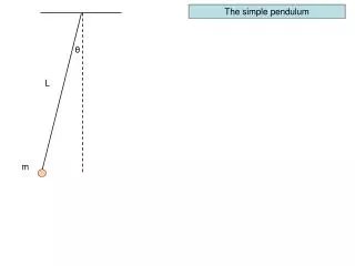
3. Parameters To Consider m-mass (or lack thereof) L-length g-gravity α-damping term I-applied torque Result: v’=-g*sin(θ)/L θ‘=v

4. Methods • Nondimensionalization • Linearization • XPP/Phase Plane analysis • Bifurcation Analysis • Theoretical Analysis

5. Nondimensionalization • Let ω=sqrt(g/L) and dτ/dt= ω • θ‘=v→v • v’=-g*sin(θ)/L →-sin(θ)

6. Systems and Equations • Simple Pendulum • θ‘=v • v‘=-sin(θ) • Simple Pendulum with Damping • θ‘=v • v‘=-sin(θ)- αv • Simple Pendulum with constant Torque • θ‘=v • v‘=-sin(θ)+I

7. Hopf Bifurcation • Simple Pendulum with Damping • θ‘=v • v‘=-sin(θ)- αv • Jacobian: • Trace=- α • Determinant=cos(θ) • Vary α from positive to zero to negative

11. The Simple Pendulum with Constant Torque and No Damping • The theta null cline: v = 0 • The v null cline: θ=arcsin(I) • Saddle Node Bifurcation I=1 • Jacobian: • θ‘=v • v‘=-sin(θ)+I

14. Driven Pendulum with Damping • θ’ = v • v’ = -sin(θ) –αv + I • Limit Cycle • The theta null cline: v = 0 • The v null cline: v = [ I – sin(θ)] / α • I = sin(θ) and as • cos2(θ) = 1 – sin2(θ) we are left with • cos(θ) = ±√(1-I2) • Characteristic polynomial- λ2 + α λ + √(1-I2) = 0 which implies λ = { ‒α±√ [α2- 4√(1-I2) ] } / 2 • Jacobian:

19. Homoclinic Bifurcation

22. Infinite Period Bifurcation

25. Bifurcation Diagram

26. Non-uniform Torque and Damped Pendulum • τ’ = 1 • θ’ = v • v’ = -sin(θ) –αv + Icos(τ)

28. Double Pendulum

29. Results Thank You! • Basic Workings Various Oscillating Systems • Hopf Bifurcation-Simple Pendulum • Homoclinic Global Bifurcation-Uniform Torque • Chaotic Behavior • Saddle Node Bifurcation • Infinite Period Bifurcation • Applications to the real world