Download
1 / 45
450 likes | 587 Views
GAs transfer through Polar Sea ice (GAPS): What we know and what we guess about air-sea exchange in ice covered waters. Brice Loose. Gas transport pathways in the ice pack. Diffusive flux. Air-sea flux. f. 1-f. How does diffusive flux compare to air-sea flux?.

E N D
GAs transfer through Polar Sea ice (GAPS): What we know and what we guess about air-sea exchange in ice covered waters Brice Loose
Gas transport pathways in the ice pack Diffusive flux Air-sea flux
f 1-f How does diffusive flux compare to air-sea flux? • Southern Ocean at 90% ice cover: • Gosink et al., (1976), Loose et al., (in press). • D = O(10-5 cm2 s-1) • - FD = 0.014 ∆C (through 50 cm of ice) • Takahashi et. al., (2009). • - FG = 1.7 ∆C pCO2 ~ 420 ppm
Thin film model Liss and Slater, 1974 • Henry’s law in the viscous sub-layer: • Cwi = HCai • leads to: • F = K(Ca-HCw) • Conductance through resistors in series: • 1/K = 1/kw + 1/ka In practice kw << ka, So K = kw
Scaling between k and open water area • Implies that k is uniquely dependent on wind/fetch k (gas transfer velocity) f 1-f 0.1 f (open water fraction)
Contents • Laboratory snapshots of k vs. open water scaling relationship. • Field estimates of k (there are only two). • Serial resistance to ocean-atmosphere exchange. • Robin boundary condition • Sensitivity example: CO2 in the Southern Ocean Seasonal Ice Zone • How to parameterize k for the ice pack? • Turbulent energy dissipation • Kinetic energy balance • Effects of stratification
Freeze experiments at CRREL • Control volume measurements: • SF6 - evasion from the water • O2 - evasion and invasion • Well-mixed tank: • Windless gas-exchange condition
Field estimates of k in ice cover. • Fanning and Torres, 1991 • 222Rn:226Ra activity, Barents Sea, 1986, 1988 • Late winter, f ~ 0.1. k = 1.4 m d-1 • Late summer, f > 0.3. k = 2.8 m d-1 • Takahashi et. al., 2009 (hypothesis) • Open ocean k ~ 3.7 m d-1 • Winter, f =0.1, k = 0.37 m d-1
Field estimates of k in ice cover. Ice Station Weddell, 1992
Field estimates of k in ice cover. Ice Station Weddell, 1992
Isopycnal tracer inventory • Mass balance between isopycnal and the surface. • M = 3He, CFC-11, S and water • Solved for k (and FCDW, ML ) Ocean surface ML Isopycnal surface FCDW
k from tracer inventory • Day 123-142: f < 0.04, k = 0.16 m d-1 • Day 143 -148: • f = 0.17, k = 0.31 m d-1
Serial resistance to ocean-atmosphere exchange Xatm Surface renewal model Equate: Ocean surface C L
Serial resistance to ocean-atmosphere exchange Xatm Surface renewal model Equate: Ocean surface C L
Serial resistance to ocean-atmosphere exchange Ice-cover (winter) Ice-free (summer) Ocean surface 100 m 100 m D = 4.3 m2d-1 D = 4300 m2d-1
3. Sensitivity example: CO2 in the Southern Ocean seasonal ice zone (SIZ)
Seasonal forcing in a transport model • Three scenarios: • S1 - k f • S2 - k f0.5 • S3 - k = CTE C = Dissolved inorganic carbon Z = depth D (10-3 m2s-1)
Primary Production • Primary prod. curve • Integrates to 57 g C m-2yr-1 • (Arrigo et al., 2008) pCO2 and DIC at the air-sea interface
Marginal ice zone • Region of ocean surface exposed in past 30 days • SO - Accounts for ~ 9% of annual primary production. Arrigo et. al., 2008
Conclusions • Sea ice cover is not sufficient to determine the value of k. • Despite ice cover, gas flux through leads accounts for 20-45% of net annual FCO2 in the seasonal ice zone. • Large gas fluxes in the spring MIZ compensate for restricted exchange during winter. We need a scaling law for k in the sea ice zone
4. How to parameterize k for the ice pack Viscosity Molecular diffusivity Zappa et al., (2007) Turbulence dissipation
4. How to parameterize k for the ice pack? Buoyant convection/stratification Ice/water current shear Wind-driven shear
4. How to parameterize k for the ice pack? [Tennekes and Driedonks, 1981] Winter mixed-layer: Spring Melt (stratification):
4. How to parameterize k for the ice pack? [Tennekes and Driedonks, 1981] Winter mixed-layer: Spring Melt (stratification):
January 2011-2013 • GAPS: (Gas Transfer through Polar Sea ice).
Spring 2011 • BRAS D’OR LAKES: In situ measurements of biological production and air-sea gas exchange during ice melt.
Spring 2011 • BRAS D’OR LAKES: In situ measurements of biological production and air-sea gas exchange during ice melt. • Quantification of biological production associated with ice melting in a “natural laboratory” that serves as an analogy of the MIZ. • Development of a method for simultaneously measuring air-sea gas exchange and biological production in ice melt zones from simple platforms.
Spring 2011 • Surface Process Instrument Platform
Acknowledgements • Postdoc Advisor - Bill Jenkins • Thesis Advisor - Peter Schlosser • Collaborators/Contributors - Wade McGillis, Stan Jacobs, Martin Stute, Juerg Matter, Chris Zappa, Eugene Gorman, Philip Orton, Bob Newton, Anthony Dachille, Tom Protus and Bernard Gallagher. • At CRREL: Don Perovich, Jackie Richter-Menge, Chris Polashenski, Bruce Elder, David Ringelberg, Mike Reynolds. • Support: NSF IGERT Fellowship, NSF AnSlope Program, LDEO Climate Center, US SOLAS Program.
CO2 Flux from SIZ • S1: 2.3 g C m-2 month-1 • S2: 2.8 g C m-2 month-1 • S3: 3.9 g C m-2 month-1
Primary Production • Primary prod. Curve • Integrates to 57 g C m-2yr-1 • (Arrigo et. al., 2008)
Processes folded into bulk diffusion rate • Molecular diffusion in liquid phase • Molecular diffusion in gas phase • Gas advection via liquid transport • Solubility partitioning between liquid and gas • Sorption onto soil grains