Download
1 / 20
220 likes | 543 Views
Anharmonic Oscillator Derivation of Second Order Susceptibilities. The harmonic oscillator model used for deriving the linear susceptibility can be extended to t he second order susceptibility. BUT, it does not agree in some details with the quantum

E N D
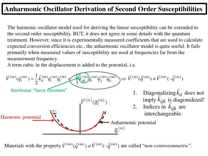
Anharmonic Oscillator Derivation of Second Order Susceptibilities The harmonic oscillator model used for deriving the linear susceptibility can be extended to the second order susceptibility. BUT, it does not agree in some details with the quantum treatment. However, since it is experimentally measured coefficients that are used to calculate expected conversion efficiencies etc., the anharmonic oscillator model is quite useful. It fails primarily when measured values of susceptibility are used at frequencies far from the measurement frequency. A term cubic in the displacement is added to the potential, i.e. Diagonalizingdoes not imply is diagonalized! Indices in are interchangeable. Nonlinear “force constant” Harmonic potential Anharmonic potential Materials with the property are called “non-centrosymmetric”.
Nonlinear Displacement (Type 1) Nonlinear “Driven” SHO Equation: Equation cannot be solved exactly -use successive approximations (1) (2) • Solve for neglecting terms • Use solutions for to evaluate • Solve for etc. Harmonic generation DC response
Nonlinear Second Harmonic Polarization: Type 1 Similarly for the DC term
Non-resonant Properties of (2)
a=c-b c=a+b b=c-a Nonlinear (Type 2) Displacements (1) Type 2 refers to 2 different eigenmodes (different polarizations, different frequencies) mixed inside a crystal. Usually refers to two orthogonally polarized fundamental beams, or to different frequencies of arbitrary polarization. The usual implementation of the first case is: E Most general case y 450 x Difference frequency generation - Sum frequency generation - Type 2 SHG for a=b orthogonally polarized beams
Type 2 Second Harmonic Generatiion e.g. 2 fundamental beams polarized along orthogonal eigenmode axes, e.g. x and y Type II Type I Type II
Non-resonant case y x - - - - - - Origin of Nonlinearity in KDP (KH2PO4) PO bonds give nonlinearity PO4 forms tetrahedron Applied Field Electron trajectory induced dipole 1 complete cycle of optical field 2 cycles of polarization to incident field
Integral Formulation of Susceptibilities Fourier component of field in frequency domain Identifies frequency for expansion in time domain
Total incident field at time Total incident field at time Second Order Susceptibility
Substituting: General Result for Total Input Fields Ensures energy conservation, e.g. Single Input Fundamental for SHG
Tedious but straight-forward Smi Single eigenmode input Exactly the same as we assumed before!
Sum and Difference Susceptibilities beams input with 2 different frequencies → 2 eigenmode input Get SHG (2aand 2b) and DC like before Focus here on a b.
where is a weak perturbation like . Assume that the complex amplitude of a generated wave varies slowly with z, i.e. is small over a wavelength. Assume CW (or long pulsed) fields, Slowly Varying Envelope Approximation (SVEA) A simple method is needed to find the fields generated by the nonlinear polarizations However, it is not always possible to solve the wave equation in matter with arbitrary polarization source terms. We will now develop a formalism in which the fields generated by perturbations can be easily calculated, provided that the perturbations are weak. It is called the Slowly Varying Envelope Approximation SVEA, sometimes called the Slowly Varying Phase and Amplitude Approximation. It involves performing an integral instead of solving a differential equation which can always be done numerically. neglect
Aside: In more general case (short pulses) with e.g. application to linear optics, dilute gas, i.e. 1>>(1) (gas density) This is a very useful result. It has been used for other small perturbations such as the acousto-optic effect, electro-optic effect, scattering by molecular vibrations etc. Note that a specific spatial Fourier component of the perturbation polarization, i.e. at kpis explicitly assumed. This approach is equivalent to first order perturbation theory in quantum mechanics.
multiply both sides by Example: SHG with 1 eigenmode input Second Harmonic Coupled Wave Equations VNB: Also valid for circular polarization!
2 DFG: 2- So far the depletion of the input beams has been neglected Down-conversion Up-conversion Both processes optimized simultaneously for wave-vector matching!
Recall: 2 Example: SHG with 2 eigenmode (polarization) inputs Therefore in the limit of Kleinman symmetry, all deffare equivalent (equal)!! It corresponds to being far off-resonance, i.e. non-resonant. Down-conversion Up-conversion
E.g. Sum (SFG) and Difference (DFG) Frequency Generation All 3processes optimized simultaneously