Download
1 / 4

E N D
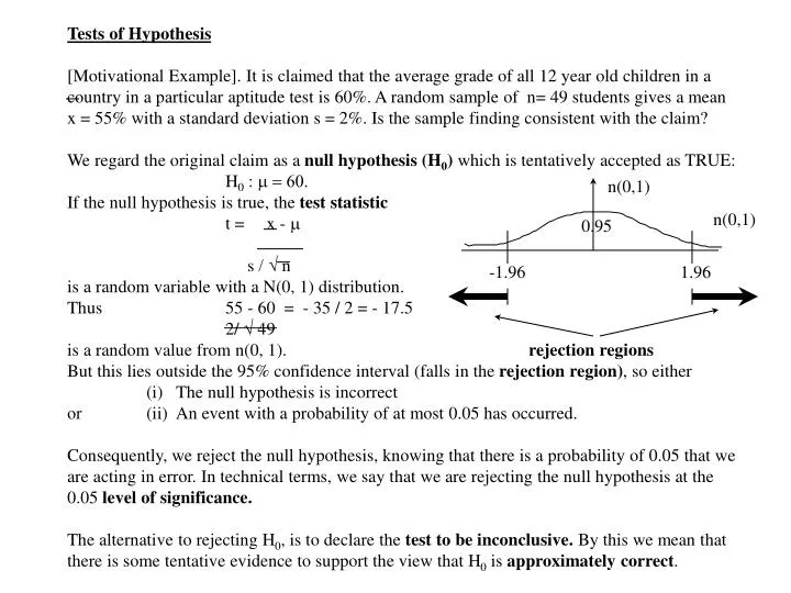
Tests of Hypothesis[Motivational Example]. It is claimed that the average grade of all 12 year old children in a country in a particular aptitude test is 60%. A random sample of n= 49 students gives a mean x = 55% with a standard deviation s = 2%. Is the sample finding consistent with the claim? We regard the original claim as a null hypothesis (H0) which is tentatively accepted as TRUE: H0 : m = 60.If the null hypothesis is true, the test statistict = x - ms / Ö nis a random variable with a N(0, 1) distribution.Thus 55 - 60 = - 35 / 2 = - 17.5 2/ Ö 49 is a random value from n(0, 1). rejection regionsBut this lies outside the 95% confidence interval (falls in the rejection region), so either (i) The null hypothesis is incorrector (ii) An event with a probability of at most 0.05 has occurred.Consequently, we reject the null hypothesis, knowing that there is a probability of 0.05 that we are acting in error. In technical terms, we say that we are rejecting the null hypothesis at the 0.05 level of significance.The alternative to rejecting H0, is to declare the test to be inconclusive. By this we mean that there is some tentative evidence to support the view that H0 is approximately correct. n(0,1) n(0,1) 0.95 -1.96 1.96
ModificationsBased on the properties of the Normal , student t and other distributions, we can generalise these ideas. If the sample size n < 25, we should use a tn-1 distribution. We can also vary the level of significance of the test and we can apply the tests to proportionate sampling environments.Example. 40% of a random sample of 1000 people in a country indicate satisfaction with government policy. Test at the .01 level of significance if this consistent with the claim that 45% of the people support government policy?Here, H0: P = 0.45 p = 0.40, n = 1000 so Ö p (1-p) / n = 0.015 test statistic = (0.40 - 0.45) / 0.015 = - 3.3399% critical value = 2.58 so H0 is rejected at the .01 level of significance.One-Tailed TestsIf the null hypothesis is of the form H0 : P ³ 0.45 then arbitrary large values of p are acceptable, so that the rejection region for the test statistic lies in the left hand tail only.Example. 40% of a random sample of 1000 people in a country indicate satisfaction with government policy. Test at the .05 level of significance if this consistent with the claim that at least 45% of the people support government policy?Here the critical value is -1.64, so thethe null hypothesis H0: P ³ 0.45 is rejected at the .05 level of significance N(0,1) 0.95 -1.64 Rejection region
Testing Differences between MeansSuppose that x1 x2 … xm is a random sample with mean x and standard deviation s1drawn from a distribution with mean m1 and y1 y2 … yn is a random sample with mean y and standard deviation s1drawn from a distribution with mean m2. Suppose that we wish to test thenull hypothesis that both samples are drawn from the same parent population (i.e.) H0: m1 = m2. The pooled estimate of the parent variance is s2 = { (m - 1) s12 + (n - 1) s22 } / ( m + n - 2)and the variance of x - y, being the variance of the difference of two independent random variables, iss ’ 2 = s2 / m + s2 / n.This allows us to construct the test statistic, which under H0 has a tm+n-2 distribution.Example. A random sample of size m = 25 has mean x = 2.5 and standard deviation s1 = 2, while a second sample of size n = 41 has mean y = 2.8 and standard deviation s2 = 1. Test at the .05 level of significance if the means of the parent populations are identical.Here H0 : m1 = m2 x - y = - 0.3 and s 2 = {24(4) + 38(1)} / 64 = 2.0938so the test statistic is - 0.3 / Ö (2.0938 / 25 + 2.0938 / 41) = - .817The .05 critical value for N(0, 1) is 1.96, so the test is inconclusive.
Paired TestsIf the sample values ( xi , yi ) are paired, such as the marks of students in two examinations, then let di = xi - yi be their differences and treat these values as the elements of a sample to generate a test statistic for the hypothesis H0: m1 = m2.The test statistic d / sd /Ö n has a tn-1 distribution if H0 is true.Example. In a random sample of 100 students in a national examination their examination mark in English is subtracted subtracted from their continuous assessment mark, giving a mean of 5 and a standard deviation of 2. Test at the .01 level of significance if the true mean mark for both components is the same.Here n = 100, d = 5, sd /Ö n = 2/10 = 0.2so the test statistic is 5 / 0.2 = 10.the 0.1 critical value for a N(0, 1) distribution is 2.58, so H0 is rejected at the .01 level of significance.Tests for the Variance.For Normally distributed random variables, given H0: s2 = k, a constant, then (n-1) s2 / k has a c 2n - 1 distribution.Example. A random sample of size 30 drawn from a normal distribution has variance s2 = 5.Test at the .05 level of significance if this is consistent with H0 : s2 = 2 .Test statistic = (29) 5 /2 = 72.5, while the .05 critical value for c 229 is 45.72, so H0 is rejected at the .05 level of significance.