Download

1 / 94
950 likes | 1.06k Views
Review of yesterday. Mini-reports. Do check the example file. Name the file appropriately. Give a suitable informative title. Write short introduction with own words. Focus on biology Write the result as statements (backup with t,p,n). (how non-sign?) Use two significance digits.

E N D
Mini-reports • Do check the example file. • Name the file appropriately. • Give a suitable informative title. • Write short introduction with own words. • Focus on biology • Write the result as statements (backup with t,p,n). (how non-sign?) • Use two significance digits. • Interpret the results in the discussion (biologically, not statistically).
Consider • Use cex, cex.lab, cex.axis! • Cred to Peter who found the cex.names. • Use ?barplot to get help.
16 14 12 10 8 6 4 Red ants Black ants Logistic regression 2 2 tables Categoric 1.0 Melica 0.8 0.6 Prob. of choosing Melica 0.4 0.2 0.0 Response variable Luzula 4.5 5.5 6.5 7.5 Ant size Regression Anova t-test Continuous - - Seed size Continuous Categoric Explanatory variable
You now can test a lot! • Most cases with: • 1 response • 1 explanatory • Today: • Summarize • Add some more technical issues • Tomorrow: • 2 explanatory variables
Binomial test binom.test(18,20) Exact binomial test data: 18 and 20 number of successes = 18, number of trials = 20, p-value = 0.0004025 alternative hypothesis: true probability of success is not equal to 0.5 95 percent confidence interval: 0.6830173 0.9876515 sample estimates: probability of success 0.9
2x2 Fisher Test fisher.test(naildata) Fisher's Exact Test for Count Data data: naildata p-value = 0.5006
Logistic regression mod.glm<-glm(Y.N~Length,binomial) anova(mod.glm,test=”Chi”) Df Deviance Resid. Df Resid. Dev P(>|Chi|) NULL 46 64.109 Length 1 1.855 45 62.254 0.173
Regression Ash seeds
Regression mod.reg<-lm(falltime~seedlength) summary(mod.reg) Coefficients: Estimate Std. Error t value Pr(>|t|) (Intercept) 1.55923 0.65656 2.375 0.024 * seedlength 0.02933 0.01905 1.540 0.13
Risk of by chance only > 5 % 95% 70 60 50 40 Normal probability 30 2,5% 2,5% 20 10 0 Difference
Risk by chance = 6.5 +6.5 = 13 % 70 60 50 40 Normal probability 30 6.5% 6.5% 20 10 0 Difference
Regression mod.reg<-lm(falltime~seedlength) summary(mod.reg) Coefficients: Estimate Std. Error t value Pr(>|t|) (Intercept) 1.55923 0.65656 2.375 0.024 * seedlength 0.02933 0.01905 1.540 0.13
Regression: a glimpse under the hood • Does x affect y? • Does the slope differ from zero?
Or in R: summary(lm(y~x))
Regression terminology • b = slope of the line • intercept = where the line cuts the y-axis • r = correlation coefficienten • = slope if you standardise y and x • ≈ how tight the points are in relation to the line. • From -1 to 1. 1=supertight positive relationship0=shutgun / no relationship • R2 = r2 = % of variation in the y-variable that is explained by the x-variable
b = 0,16 sec / mm p = 0.013 fall time ~ wing length
r = 0,56 R2 = 0,31 r n p = 0,013 standardised fall time ~ standardised wing length
t-test table t.test(twiglength~treeside,var.equal=T) Two Sample t-test t = -2.7427, df = 38, p-value = 0.009244 mean in group shade mean in group sunny 1.475 2.705
Confidence intervals • …shows how sure we are of a group mean. • The confidence interval will contain the ”true” mean in 95 % of the time. • The larger our sample size the more sure (= confident!) we are of our sample mean the confidence interval decreases • And (of course…), the more variation within groups, the less sure we get confidence interval increases
Is there any difference? Seed size in plants
t-test table t.test(twiglength~treeside,var.equal=T) Two Sample t-test t = -2.7427, df = 38, p-value = 0.009244 mean in group shade mean in group sunny 1.475 2.705
Anova mod.aov<-aov(twiglength~treeside) summary(mod.aov) Df Sum Sq Mean Sq F value Pr(>F) treeside 1 15.129 15.129 7.5222 0.009244 ** Residuals 38 76.427 2.011
How does this F-test work? • The idea behind the F-test is to check whether the variation caused by the explanatory variable is larger than the random variation in each data point. • In this case the variation caused by the explanatory variable is the variation among groups. • The random variation is simply the variation that is NOT explained by the explanatory variable.
How does this F-test work? • Under the hood. • A frog example. female male
We measure 4 + 4 frogs 10 15 12 14 8 11 9 7