Download
1 / 17
220 likes | 658 Views
CS203 – Advanced Computer Architecture. Dependability & Reliability. Failures in Chips. Transient failures (or soft errors) Charge q = c*v if c and v decrease then it is easier to flip a bit Sources are cosmic rays and alpha particles and electrical noise

E N D
CS203 – Advanced Computer Architecture Dependability & Reliability
Failures in Chips • Transient failures (or soft errors) • Charge q = c*v if c and v decrease then it is easier to flip a bit • Sources are cosmic rays and alpha particles and electrical noise • Device is still operational but value has been corrupted • Intermittent/temporary failures • Last longer • Due to • Temporary: environmental variations (eg, temperature) • Intermittent: aging • Permanent failures • Means that the device will never function again • Must be isolated and replaced by spare • Process variations increase the probability of failures
Define and quantify dependability • Reliability = • measure of continuous service accomplishment (or time to failure). • Metrics • Mean Time To Failure (MTTF) measures reliability • Failures In Time (FIT) = 1/MTTF, the rate of failures • Traditionally reported as failures per 109 hours of operation • Ex. MTTF = 1,000,000 FIT = 109/106 = 1000 • Mean Time To Repair (MTTR) measures Service Interruption • Mean Time Between Failures (MTBF) = MTTF+MTTR
Define and quantify dependability • Availability = • measures service as alternate between the 2 states of accomplishment and interruption (number between 0 and 1, e.g. 0.9) • Module availability = MTTF / ( MTTF + MTTR)
Fault-Tolerance • How to measure a system’s ability to tolerate faults? • Reliability = Probability[no failure @ time t] = R(t) • Availability = Probability[system operational] • E.g. AT&T ESS-1, one of the first computer-controlled telephone exchange (deployed in 1960s) was designed for less than two hours of downtime over its lifetime: 40 years. Availability = 99.9994% • Failure rate • Fraction of samples that fail per unit time • Is NOT constant, changes over time • R(t) = N(t)/N(0), where N(t) is the number of operational units at time t.
Example calculating reliability • If modules have exponentially distributed lifetimes (age of module does not affect probability of failure), • Overall failure rate is the sum of failure rates of all the modules • Calculate FIT and MTTF for 10 disks (1M hour MTTF per disk), 1 disk controller (0.5M hour MTTF), and 1 power supply (0.2M hour MTTF):
1 3 2 Early Life Region Wear-Out Region Constant Failure Rate Region The“Bathtub” Curve Failure Rate 0 Time t
1 Early Life Region The “Bathtub” Curve Burn-in is a test performed to screen or eliminate marginal components with inherent defects or defects resulting from manufacturing process. Failure Rate 0 Time t
2 Constant Failure Rate Region The “Bathtub” Curve An important assumption for effective maintenance is that components will eventually have an Increasing Failure Rate. Maintenance can return the component to the Constant Failure Region. Failure Rate 0 Time t
3 Wear-Out Region The “Bathtub” Curve Components will eventually enter the Wear-Out Region where the Failure Rate increases, even with an effective Maintenance Program. You need to be able to detect the onset of Terminal Mortality Failure Rate 0 Time t
Derivation of R(t) • Probability[no failure @ time t] = R(t) • Assuming a constant failure rate λ, N is the number of units Integrating with R(0) = 1 boundary: R(t) = e-λt
System Reliability • Series system • Parallel system R1 R1 R2 Rn R2 Rn
Triple Modular Redundancy • TMR: Triple Modular Redundancy • three concurrent devices plus a voter (assume no voter failure) • RTMR(t) = R3(t) + 3R2(t)(1 – R(t)) = 3R2(t) – 2R3(t) • Let R(t) = e-λt, then RTMR = 3e-2λt – 2e-3λt Voter Result
Simplex v/s TMR Reliability TMR has higher reliability for short mission times Reliability After 1st failure, TMR equivalent to 2 component in series λt
MTTF - Mean-Time To Failure Let F(t) = 1 – R(t), the failure probability (cdf) and f(t) = dF(t)/dt, the failure probability density Expected working life of a unit with an exponentially distributed reliability is the inverse of its failure rate
MTBF • The MTBF is widely used as the measurement of equipment's reliability and performance. • This value is often calculated by dividing the total operating time of the units by the total number of failures encountered. • This metric is valid only when the data is exponentially distributed. • This is a poor assumption which implies that the failure rate is constant if it is used as the sole measure of equipment's reliability.
Summary • How to define dependability • How to quantify dependability • How to measure Reliability of a system