Download
1 / 24
240 likes | 297 Views
On the spectrum of Hamiltonians in finite dimensions. Roberto Oliveira. Joint with David DiVincenzo and Barbara Terhal @ IBM Watson. Paraty, August 14 th 2007. In one slide: Ground state energy is hard. Bulk of the spectrum is Gaussian and universal. The setup.

E N D
On the spectrum of Hamiltonians in finite dimensions Roberto Oliveira Joint with David DiVincenzo and Barbara Terhal @ IBM Watson. Paraty, August 14th 2007.
In one slide:Ground state energy is hard.Bulk of the spectrum is Gaussian and universal.
The setup • H = Hamiltonian on a set V of N spin ½ particles. • Spec(H) = {0·1·2…}. • We will assume Tr(H)=0. • 2(H) = “variance” = Tr(H2)/2N • Write H = X½ V HX , • where HX acts on the spins in X. Can assume Tr(HXHY)=0 if X Y.
E.g.: Ising with transverse field H = (bond terms) + (site terms) bond term H{i,j} = J xx[i,j] i j k site term H{k} = h z[k] H=k H{k} + i~jH{i,j}
E.g.: Ising with transverse field face term HF H = (bond terms) + (site terms) bond term H{i,j} = J xx[i,j] i j k site term H{k} = h z[k] H=k H{k} + i~jH{i,j} + FHF
Dimensionality assumption • 9metric and d, C, c, >0 such that: Radius R cRd·X½B(x,R)2(HX)·CRd X½ B(x,R)||HX||·CRd center x X ½ B(x,R)2(HX)·CRd- B(x,R) = {v2 V : (v,x)· R}
E.g. nearest neighbor in Zd Radius R • L1 norm • ¼ Rd terms inside • ¼ Rd-1 at the boundary
Gaussian spectrum • Plot a histogram of Spec(H/(H)). • with small but fixed bin size b>0. That will approach • a Gaussian as N adiverges, for fixed parameters.
A bit more formally • There is a probability measure on the line given by H: • m=H= 2-N2 Spec(H) • We show that this measure is approximately normal in the sense that for all a<b, as N grows: • H (a(H),b(H)) !(2)-1/2sab exp(-t2/2)dt
Even more formally • Recall: strength inside ball ¼Rd,strength across boundary ¼ Rd-, with C,c extra parameteres. • Then for all a<b, • |H [a(H),b(H)]-(2)-1/2sab exp(-t2/2)dt| • · D(C,c,d,) (Diam())-d/8
A bit less formally again • Inside ¼ Rd, boundary¼ Rd-. Radius R H/(H)[x,y] ¼ (2)-1/2sxy exp(-t2/2)dt center x B(x,R) = {v2 V : (v,x)· R}
A simple case • We will now explain a special case of the Theorem. • Nearest neighbor interactions on a n x n patch of the planar square lattice (N=n2 spins). • Also assume that all terms in the Hamiltonian have norm of constant order.
Back to that old slide H = (bond terms) + (site terms) bond term H{i,j} = J xx[i,j] i j k site term H{k} = h z[k] H=k H{k} + i~jH{i,j}
What do we do? • Main idea: ignore terms acting on red lines (i.e. treat non-interacting systems). Then put them back in via a perturbation argument.
Omitting the interactions • G = s Gs, subsystems might have high dimension. • How does one compute the global spectrum? Answer: convolution of the individual spectral distributions. • By the usual Central Limit Theorem, G/(G) is approximately Gaussian as long as some conditions are satisfied.
Which conditions? • Many terms in the sum. • The influence of any given term is small. • m¿ n1/2 suffices.
Next step • Recall that we have. • H/(H) = 2-N2 Spec(H) /(H) • We know that G/(G) is approx. gaussian. • G/(G) = 2-N2 Spec(G) /(G) • We will show that (H-G) is small. • By a perturbation theory argument, this implies that H/(H)¼ G/(G).
(H-G) is small • Variance¼ # of qubits • Total # of qubits ¼ n2 • Qubits on red lines ¼ m(n/m)2 = n2/m • ) (H-G)2·(H)2/m, small if mÀ 1
To conclude • Take some 1¿ m¿ n1/2 (e.g. m=n1/3). • Then G/(G) is approx. Gaussian. • Also H/(H)¼ G/(G). So we are done. • The key step: m x m boxes have m2 vertices but only ¼ m vertices on their boundaries.
General case • Inside ¼ Rd, boundary¼ Rd-. Radius R H/(H)[a,b] ¼ (2)-1/2sab exp(-t2/2)dt center x B(x,R) = {v2 V : (v,x)· R}
General result: proof sketch • Main idea: break the system into subparts with small total boundary strength. • Treat isolated systems via standard CLT. • Put the boundary back in via perturbation theory.
Conclusions • Spectral distribution is approximately Gaussian with std. deviation ¼ N1/2. • This is universal for quantum spin systems in finite dimensional structures when long-range interactions decay fast enough.
Further work • Bounds are actually weak for many problems. Are there better bounds for specific systems? • Fermions? Bosons? • Applications?