Download
1 / 22
220 likes | 355 Views
Summer Project Presentation. Presented by:Mehmet Eser Advisors : Dr. Bahram Parvin Associate Prof. George Bebis. Introduction. What is morphing ? In what areas is morphing used ? What methods are used for morphing for solid shapes?. What are Solid Shapes?. A slice from a brain MRI scan.

E N D
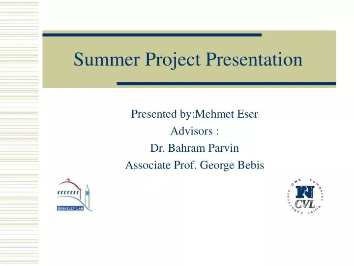
Summer Project Presentation Presented by:Mehmet Eser Advisors : Dr. Bahram Parvin Associate Prof. George Bebis
Introduction • What is morphing ? • In what areas is morphing used ? • What methods are used for morphing for solid shapes? Lawrence Berkeley National Laboratory & UNR Computer Vision Laboratory
What are Solid Shapes? A slice from a brain MRI scan Extracted & Rendered Isosurface Lawrence Berkeley National Laboratory & UNR Computer Vision Laboratory
Problem Definition • Interpolation of solid shapes Let S be a deformable closed surface such that a family of evolved surfaces with initial conditions at • Construct intermediate solid shapes satisfying smoothness and continuity in time Lawrence Berkeley National Laboratory & UNR Computer Vision Laboratory
Approach to The Problem • Defining the intermediate interpolated shapes implicitly: such that The givens of the problem Lawrence Berkeley National Laboratory & UNR Computer Vision Laboratory
Regularization Method • A numerical solution method • Applied to the ill-posed problems • The original problem is converted into a well-posed problem by satisfying some smoothness constraint. • A smoothing parameter which controls the trade-off between an error term and the the amount of smoothing (regularization) Lawrence Berkeley National Laboratory & UNR Computer Vision Laboratory
t=0.2 Gradients can be helpful? Lawrence Berkeley National Laboratory & UNR Computer Vision Laboratory
Approach to The Problem • Gradients can be used for finding a unique solution to the problem • Disadvantages of this approach • Global average may be small • But locally gradient of f may change sharply (not good for a smooth interpolation of curves) Lawrence Berkeley National Laboratory & UNR Computer Vision Laboratory
Purposed Method • Minimization of the supremum of the • For minimization of the supremum of the gradients of the functions sup can be written as follows (in series): Lawrence Berkeley National Laboratory & UNR Computer Vision Laboratory
Purposed Method • The minimization of this function can be achieved by using the Euler equation • The result of the min of is the following Lawrence Berkeley National Laboratory & UNR Computer Vision Laboratory
Implementation • Distance Field Transforms • Finding an approximation to the problem with Distance Field Transform. • Employing the regularization term • Generation of the Morphing Lawrence Berkeley National Laboratory & UNR Computer Vision Laboratory
Distance Transformation • Distance Transformations • Obtained in time for 3D D(x,y,z) Lawrence Berkeley National Laboratory & UNR Computer Vision Laboratory
An example to Distance Transform Original Image Distance Image Lawrence Berkeley National Laboratory & UNR Computer Vision Laboratory
DT’s of a Cube and a Sphere A slice of a distance transformed cube A slice of a distance transformed sphere Lawrence Berkeley National Laboratory & UNR Computer Vision Laboratory
Signed Distance Transform • Calculation of signed distance transform • Take negative of the distance value if the pixel is inside the object • Take positive of the distance value if the pixel is outside the object • Morphing region is defined as Lawrence Berkeley National Laboratory & UNR Computer Vision Laboratory
Interpolation Region Lawrence Berkeley National Laboratory & UNR Computer Vision Laboratory
C1 Vi S Q P V0 B A R V1 V0 Interpolating Surfaces Lawrence Berkeley National Laboratory & UNR Computer Vision Laboratory
Why Distance Field ? • A smooth and natural interpolation of surfaces • Can be carried out at any desired resolution • A good initial seed for the iteration with ILE • PDE ‘s can be calculated finite difference formulas Lawrence Berkeley National Laboratory & UNR Computer Vision Laboratory
Numerical Solution to ILE • Get the interpolated surfaces • Iterate using regularization term-ILE • v iteration number • step size • F interpolated volume Lawrence Berkeley National Laboratory & UNR Computer Vision Laboratory
Iteration 1.Initialize F with boundary conditions 2.Initialize R with the approximated morphing 3.Update all points inside R with equation (1) 4.Compute 5.Repeat 3 & 4 till the local minimum of sup|F| is reached. 6.Obtain morphed volumes S(t) = {(x,y,z,) | F(x,y,z) = t } Lawrence Berkeley National Laboratory & UNR Computer Vision Laboratory
Results Lawrence Berkeley National Laboratory & UNR Computer Vision Laboratory
Special Thanks to National Science Foundation (NFS) UNR Computer Vision Laboratory (Assoc. Prof. George Bebis lead) LBL Vision Group (Dr. Bahram Parvin lead)