Download
1 / 15
160 likes | 283 Views
Design and Implementation of VLSI Systems (EN1600) Lecture 18: Scaling Theory . Prof. Sherief Reda Division of Engineering, Brown University Spring 2008. [sources: Weste/Addison Wesley – Rabaey/Pearson]. IBM Cell. 234M transistors in die size of 221 mm 2. Moore’s Law.

E N D
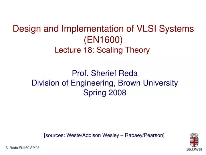
Design and Implementation of VLSI Systems (EN1600) Lecture 18: Scaling Theory Prof. Sherief Reda Division of Engineering, Brown University Spring 2008 [sources: Weste/Addison Wesley – Rabaey/Pearson]
IBM Cell 234M transistors in die size of 221 mm2 Moore’s Law Moore’s Law. The number of transistors in an integrated circuit doubles every 2 years.
Scaling of MOS transistors 1.2nm minimum feature size (gate length) Current oxide thickness ~ 1.0 – 2.0nm thickness 3 – 4 atomic layers of oxide Power supply voltage scaling
Scaling of lithographic wavelength Scaling Avg transistor priceis 0.1 μcent! Fewer and fewer companies can afford to have their own foundries Number of transistors shipped
Device scaling (very idealistic NMOS transistor) (scaled down by L) scale doping increased by a factor of S Increasing the channel doping density decreases the depletion width improves isolation between source and drain during OFF status permits distance between the source and drain regions to be scaled
Historically frequency scaled by more than S • Intel VP Patrick Gelsinger (ISSCC 2001) • “If scaling continues at present pace, by 2005, high speed processors would have power density of nuclear reactor, by 2010, a rocket nozzle, and by 2015, surface of sun.”
Scaling of standby (leakage) power bottleneck Standby power • Even if Vt is kept constant after scaling, Poff scales up by S if tox is scaled down by S • Vt must be scaled down if VDD is scaled down (otherwise ISAT is weaker and transistor is slow) • Standby power would further increase by 10 for every 0.1V reduction of Vt
higher active power increasing performance higher leakage Power/performance tradeoffs Power supply voltage (Vdd) Threshold voltage (Vt) [Taur, 01]
Interconnect scaling w: width of interconnect (layer dependant) s: spacing between interconnects with same layer h: dielectric thickness (spacing between interconnects in two vertically adjacent layers) l: length of interconnect t: thickness of interconnect
Constant thickness scaling versus reduced thickness scaling constant thickness scaling reduced thickness scaling
Interconnect delay is dominating gate delay bottleneck Repeaters can help but…
With scaling the reachable radius of a buffer decreases we need more and more buffers bottleneck repeaters required to buffer Itanium global interconnects • A corner-to-corner (BL-UR) wire in Itanium (180nm) requires 6 repeaters to span die • Repeaters consume chip area; consume power; add vias
Done with chapter 4: Delay estimation Power estimation Interconnects and wire engineering Design Margins Scaling theory Summary