Download
1 / 103
1.22k likes | 1.55k Views
Introduction to Mobile Robots Motion Planning. Prof.: S. Shiry Pooyan Fazli M.Sc Computer Science Department of Computer Eng. and IT Amirkabir Univ. of Technology (Tehran Polytechnic). What is Motion Planning?. Determining where to go. The World consists of. Obstacles

E N D
Introduction to Mobile Robots Motion Planning Prof.: S. Shiry Pooyan Fazli M.Sc Computer Science Department of Computer Eng. and IT Amirkabir Univ. of Technology (Tehran Polytechnic)
What is Motion Planning? • Determining where to go
The World consists of... • Obstacles • Already occupied spaces of the world • In other words, robots can’t go there • Free Space • Unoccupied space within the world • Robots “might” be able to go here • To determine where a robot can go, we need to discuss what a Configuration Space is
Notion of Configuration Space • Main Idea: Represent the robot as a point, called a configuration, in a parameter space, the configuration space (or C-space). • Importance: Reduce the problem of planning the motion of a robot in Euclidean Space to planning the motion of a point in C-space.
C-space of Rigid Object Robot Configurations Can be: • 1. Free configurations: robot and obstacles do not overlap • 2. Contact configurations: robot and obstacles touch • 3. Blocked configurations: robot and obstacles overlap • Configuration Space partitioned into free (Cfree), contact, and blocked sets.
Obstacles in C-space Cspace = Cfree + Cobstacle
Example of a World (and Robot) Free Space Obstacles Robot x,y
The Configuration Space • How to create it • First abstract the robot as a point object. Then, enlarge the obstacles to account for the robot’s footprint and degrees of freedom • In our example, the robot was circular, so we simply enlarged our obstacles by the robot’s radius (note the curved vertices)
Configuration Space:Accommodate Robot Size Free Space Obstacles Robot (treat as point object) x,y
Motion Planning • General Goal: compute motion commands to achieve a goal arrangement of physical objects from an initial arrangement • Basic problem: Collision-free path planning for one rigid or articulated object (the “robot”) among static obstacles. Inputs • geometric descriptions of the obstacles and the robot • kinematic and dynamic properties of the robot • initial and goal positions (configurations) of the robot Output • Continuous sequence of collision-free configurations connecting the initial and goal configurations
Motion Planning • Path planning design of only geometric (kinematic) specifications of the positions and orientations of robots • Trajectory = Path + assignment of time to points along the path • Trajectory planning path planning + design of linear and angularvelocities • Motion Planning (MP),a general term, either: • Path planning, or • Trajectory planning • Path planning < Trajectory planning
Extensions to the Basic Problem • movable obstacles • moving obstacles • multiple robots • incomplete knowledge/uncertainty in geometry, sensing, etc.
Classification of MP algorithms Completeness • Exact • usually computationally expensive • Heuristic • aimed at generating a solution in a short time • may fail to find solution or find poor one at difficult problems • important in engineering applications • Probabilistically complete (probabilistic completeness 1)
Classification of MP algorithms Scope • Global • take into account all environment information • plan a motion from start to goal configuration • Local • avoid obstacles in the vicinity of the robot • use information about nearby obstacles only • used when start and goal are close together • used as component in global planner, or • used as safety feature to avoid unexpected obstacles not present in environment model, but sensed during motion
Classification of MP Algorithms • Point-to-point • Region filling
Point-to-point Path Planning • Point-to-point path planning looks for the best route to move an entity from point A to point B while avoiding known obstacles in its path, not leaving the map boundaries, and not violating the entity's mobility constraints. • This type of path planning is used in a large number of robotics and gaming applications such as finding routes for autonomous robots, planning the manipulator's movement of a stationary robot, or for moving entities to different locations in a map to accomplish certain goals in a gaming application.
Region Filling Path Planning • Tasks such as vacuuming a room, plowing a field, or mowing a lawn require region filling path planning operations that are defined as follows: 1) The mobile robot must move through an entire area, i.e., the overall travel must cover a whole region. 2) Continuous and sequential operation without any repetition of paths is required of the robot. 3) The robot must avoid all obstacles in a region. 4) An "optimal" path is desired under the available conditions.
Motion Planning Statement • The Problem: • Given an initial position and orientation POinit • Given a goal position and orientation POgoal • Generate: continuous path t from POinit to POgoal • t is a continuous sequence of Pos’
The Wavefront Planner • A common algorithm used to determine the shortest paths between two points • In essence, a breadth first search of a graph • For simplification, we’ll present the world as a two-dimensional grid • Setup: • Label free space with 0 • Label C-Obstacle as 1 • Label the destination as 2
Representations: A Grid • Distance is reduced to discrete steps • For simplicity, we’ll assume distance is uniform • Direction is now limited from one adjacent cell to another
Representations: Connectivity • 8-Point Connectivity • 4-Point Connectivity
The Wavefront in Action (Part 1) • Starting with the goal, set all adjacent cells with “0” to the current cell + 1 • 4-Point Connectivity or 8-Point Connectivity? • Your Choice. We’ll use 8-Point Connectivity in our example
The Wavefront in Action (Part 2) • Now repeat with the modified cells • This will be repeated until no 0’s are adjacent to cells with values >= 2 • 0’s will only remain when regions are unreachable
The Wavefront in Action (Part 3) • Repeat again...
The Wavefront in Action (Part 4) • And again...
The Wavefront in Action (Part 5) • And again until...
The Wavefront in Action (Done) • You’re done • Remember, 0’s should only remain if unreachable regions exist
The Wavefront, Now What? • To find the shortest path, according to your metric, simply always move toward a cell with a lower number • The numbers generated by the Wavefront planner are roughly proportional to their distance from the goal Two possible shortest paths shown
Map-Based Approaches: Roadmap Theory • Idea: capture the connectivity of Cfree with a roadmap (graph or network) of one-dimensional curves
Roadmap Methods • Properties of a roadmap: • Accessibility: there exists a collision-free path from the start to the road map • Departability: there exists a collision-free path from the roadmap to the goal. • Connectivity: there exists a collision-free path from the start to the goal (on the roadmap). • Examples of Roadmaps • Visibility Graph • Generalized Voronoi Graph (GVG)
The Visibility Graph in Action (Part 1) • First, draw lines of sight from the start and goal to all “visible” vertices and corners of the world. goal start
The Visibility Graph in Action (Part 2) • Second, draw lines of sight from every vertex of every obstacle like before. Remember lines along edges are also lines of sight. goal start
The Visibility Graph in Action (Part 3) • Second, draw lines of sight from every vertex of every obstacle like before. Remember lines along edges are also lines of sight. goal start
The Visibility Graph in Action (Part 4) • Second, draw lines of sight from every vertex of every obstacle like before. Remember lines along edges are also lines of sight. goal start
The Visibility Graph (Done) • Repeat until you’re done. goal start
Reduced Visibility Graphs • Idea: we don't really need all the edges in the visibility graph (even if we want shortest paths) • Definition: Let L be the line passing through an edge (x,y) in the visibility graph G. The segment (x,y) is a tangent segment iff L is tangent to CB at both x and y.
Retraction Example: Generalized Voronoi Diagrams • A GVG is formed by paths equidistant from the two closest objects • This generates a very safe roadmap which avoids obstacles as much as possible