Download
1 / 34
340 likes | 442 Views
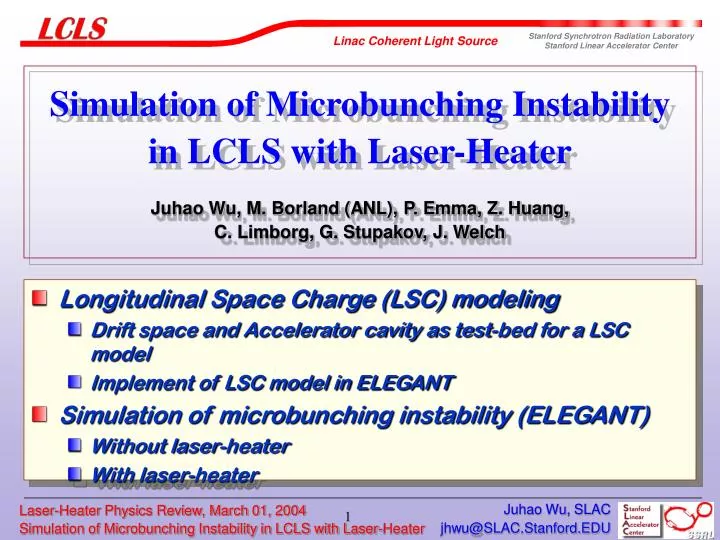
Simulation of Microbunching Instability in LCLS with Laser-Heater Juhao Wu, M. Borland (ANL), P. Emma, Z. Huang, C. Limborg, G. Stupakov, J. Welch. Longitudinal Space Charge (LSC) modeling Drift space and Accelerator cavity as test-bed for a LSC model Implement of LSC model in ELEGANT

E N D
Simulation of Microbunching Instability in LCLS with Laser-HeaterJuhao Wu, M. Borland (ANL), P. Emma, Z. Huang, C. Limborg, G. Stupakov, J. Welch • Longitudinal Space Charge (LSC) modeling • Drift space and Accelerator cavity as test-bed for a LSC model • Implement of LSC model in ELEGANT • Simulation of microbunching instability (ELEGANT) • Without laser-heater • With laser-heater Juhao Wu, SLAC
Motivation • What’s new? LSC important in photoinjector and downstream beam line; (see Z. Huang’s talk) • PARMELA / ASTRA simulation time consuming for S2E; difficult for high-frequency microbunching (numerical noise); • Find simple, analytical LSC model, and implement it to ELEGANT for S2E instability study; • Starting point –- free-space 1-D model; (justification) • Transverse variation of the impedance decoherence; small? 2-D? • Pipe wall decoherence; small? • Test LSC model in simple element • Use such a LSC model for S2E instability study Juhao Wu, SLAC
LSC Model (1-D) • Free space 1-D model: transverse uniform coasting beam with longitudinal density modulation (on-axis) • where, rb is the radius of the coasting beam; λ rb pancake beam pencil beam • For more realistic distribution find an effective rb, and use the above impedance; • Radial-dependence of the impedance will increase energy spread and enhance damping; small? Juhao Wu, SLAC
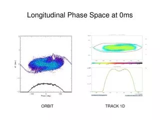
Space Charge Oscillation in a Coasting Beam • Distinguish: low energy case high energy case; • Space charge oscillation becomes slow, when the electron energy becomes high; the residual density modulation is then ‘frozen’ in the downstream beam line. rb=0.5 mm, I0=100 A E = 12 MeV E = 6 MeV Juhao Wu, SLAC
Two Quantities • The quantities we concern are density modulation, and energy modulation Heifets-Stupakov-Krinsky(PRST,2002); Huang-Kim(PRST,2002) (CSR) Density modulation Integral equation approach Energy modulation R56 Juhao Wu, SLAC
Testing the LSC model • Analytical integral equation approach • Find an effective radius for realistic transverse distributions and use 1-D formula for LSC impedance; for parabolic & Gaussian • Generalize the momentum compaction function to treat acceleration in LINAC, and for drift space as well • Simulation • PARMELA • ASTRA • ELEGANT Juhao Wu, SLAC
Integral Equations Density modulation Energy Modulation: • Applicable for both accelerator cavity and drift space • Impedance for LSC Juhao Wu, SLAC
Analytical Approach – Two Limits • Analytical integral equation approach – two limits • Density and energy modulation in a drift at distance s; • At a very large , plasma phase advance (s/c) << 1, • “frozen,” energy modulation gets accumulated • (Saldin-Schneidmiller-Yurkov, TESLA-FEL-2003-02) • Integral equation approach deals the general evolution of the density and energy modulation Juhao Wu, SLAC
Analytical vs. ASTRA (energy modulation) • 3 meter drift without acceleration • In analytical approach: • Transverse beam size variation due to transverse space charge: included; • Slice energy spread increases: not included; • 1 keV resolution? Coasting beam vs. bunched beam? Juhao Wu, SLAC
Analytical vs. ASTRA (density modulation) • 3 meter drift without acceleration Juhao Wu, SLAC
Analytical vs. PARMELA (energy modulation) • Assume 10% initial density modulation at gun exit at 5.7 MeV; • After 67 cm drift + 2 accelerating structures (150 MeV in 7 m), LSC induced energy modulation; PARMELA simulation Analytical approach Juhao Wu, SLAC
S2E Simulation • LSC model • Analytical approach agrees with PARMELA / ASTRA simulation; • Wall shielding effect is small as long as (typical in our study); • Free space calculation overestimates the results (10 – 20%); • Radial-dependence and the shielding effect decoherence; (effect looks to be small) • Free space 1-D LSC impedance with effective radius has been implemented in ELEGANT; • S2E simulation • Injector simulation with PARMELA / ASTRA (see C. Limborg’s talk); • downstream simulations ELEGANT with LSC model(CSR, ISR, Wake etc. are all included) Juhao Wu, SLAC
Comparison with ELEGANT • Free space 1-D LSC model with effective radius • Example with acceleration: current modulation at different wavelength I=100 A, rb=0.5 mm, E0=5.5 MeV, Gradient: 7.5 MV/m --- 1 mm, --- 0.5 mm, --- 0.25 mm, --- 0.1 mm Elegant tracking Analytical calculation Juhao Wu, SLAC
Simulation Details • Halton sequence (quiet start) particle generator • Based on PARMELA output file at E=135 MeV, with 200 k particles • Longitudinal phase space: keep correlation between t and p --- fit p(t), and also local energy spread p(t) • Multiply density modulation ( 1 %) • Transverse phase space: keep projected emittance • 6-D Quiet start to regenerate 2 million particles • Bins and Nyquist frequency --- typically choose bins to make the wavelength we study to be larger than 5 Nyquist wavelength • 2000 bins for initial 11.6 ps bunch • Nyquist wavelength is 3.48 m • We study wavelength longer than 20 m Juhao Wu, SLAC
Simulation Details • Wake • Low-pass filter is essential to get stable results • Smoothing algorithms (e.g. Savitzky-Golay) is not helpful • Non-linear region • Synchrotron oscillation rollover harmonics • Low-pass filter is set to just allow the second harmonic Current form-factor Low-pass filter Impedance Juhao Wu, SLAC
Simulation Details • Gain calculation (linear region) • Choose the central portion to do the analysis • Use polynomial fit to remove any gross variation • Use NAFF to find the modulation wavelength and the amplitude Juhao Wu, SLAC
Phase space evolution along the beam line • Without laser-heater ( 1% initial density modulation at 30 m ) • Really bad • With matched laser-heater ( 1% initial density modulation at 30 m ) • Microbunching is effectively damped Juhao Wu, SLAC
DE/E DE/E time (sec) time (sec) 510-5 510-5 30 mm injector output (135 MeV) 1% LCLS l0 = 30 mm NO HEATER
DE/E DE/E time (sec) time (sec) 510-5 510-5 30 mm after DL1 dog-leg (135 MeV) LCLS l0 = 30 mm NO HEATER
DE/E DE/E time (sec) time (sec) 110-3 110-3 30 mm before BC1 chicane (250 MeV) LCLS l0 = 30 mm NO HEATER
DE/E DE/E time (sec) time (sec) 110-3 110-3 30/4.3 mm after BC1 chicane (250 MeV) LCLS l0 = 30 mm NO HEATER
DE/E DE/E time (sec) time (sec) 510-4 510-4 30/4.3 mm before BC2 chicane (4.5 GeV) LCLS l0 = 30 mm NO HEATER
DE/E DE/E time (sec) time (sec) 210-3 210-3 30/30 mm after BC2 chicane (4.5 GeV) LCLS l0 = 30 mm NO HEATER
DE/E DE/E time (sec) time (sec) 110-3 110-3 0.09 % rms 30/30 mm before undulator (14 GeV) LCLS l0 = 30 mm NO HEATER
DE/E DE/E time (sec) time (sec) 510-5 510-5 30 mm injector output (135 MeV) 1% LCLS l0 = 30 mm MATCHED HEATER
DE/E DE/E time (sec) time (sec) 510-4 510-4 30 mm just after heater (135 MeV) LCLS l0 = 30 mm MATCHED HEATER
DE/E DE/E time (sec) time (sec) 510-4 510-4 30 mm after DL1 dog-leg (135 MeV) LCLS l0 = 30 mm MATCHED HEATER
DE/E DE/E time (sec) time (sec) 110-3 110-3 30 mm before BC1 chicane (250 MeV) LCLS l0 = 30 mm MATCHED HEATER
DE/E DE/E time (sec) time (sec) 210-3 210-3 30/4.3 mm after BC1 chicane (250 MeV) LCLS l0 = 30 mm MATCHED HEATER
DE/E DE/E time (sec) time (sec) 510-4 510-4 30/4.3 mm before BC2 chicane (4.5 GeV) LCLS l0 = 30 mm MATCHED HEATER
DE/E DE/E time (sec) time (sec) 510-4 510-4 30/30 mm after BC2 chicane (4.5 GeV) LCLS l0 = 30 mm MATCHED HEATER
DE/E DE/E time (sec) time (sec) 210-4 210-4 0.01% rms 30/30 mm before undulator (14 GeV) LCLS l0 = 30 mm MATCHED HEATER
LCLS gain and slice energy spread End of BC2 Nonlinear region / Saturation 1%, 30m Undulator entrance Juhao Wu, SLAC
Discussion and Conclusion • Instability not tolerable without laser-heater for < 200 -- 300 m with about 1% density modulation after injector; • Laser-heater is quite effective and a fairly simple and prudent addition to LCLS; • Injector modulation study also important, no large damping is found to confidently eliminate heater. (see C. Limborg’s talk) Juhao Wu, SLAC