Download
1 / 45
450 likes | 694 Views
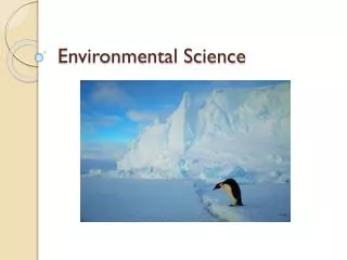
Core Case Study: Endangered Southern Sea Otter (1) . Santa Cruz to Santa Barbara shallow coastLive in kelp forestsEat shellfish~16,000 around 1900Hunted for fur and because considered competition for abalone and shellfish. Core Case Study: Endangered Southern Sea Otter (2) . 1938-2008: increase

E N D
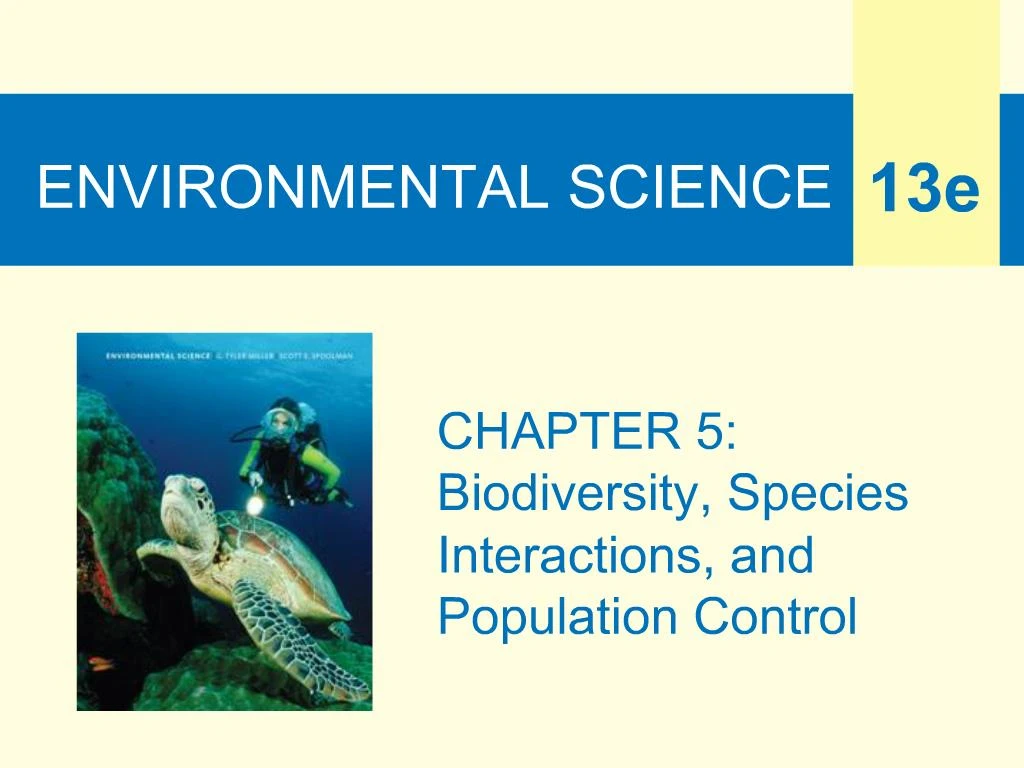
1. ENVIRONMENTAL SCIENCE
2. Core Case Study: Endangered Southern Sea Otter (1) Santa Cruz to Santa Barbara shallow coast
Live in kelp forests
Eat shellfish
~16,000 around 1900
Hunted for fur and because considered competition for abalone and shellfish
3. Core Case Study: Endangered Southern Sea Otter (2) 1938-2008: increase from 50 to ~2760
1977: declared an endangered species
Why should we care?
Cute and cuddly � tourists love them
Ethics � it�s wrong to hunt a species to extinction
Keystone species � eat other species that would destroy kelp forests
6. 5-1 How Do Species Interact? Concept 5-1 Five types of species interactions affect the resource use and population sizes of the species in an ecosystem.
7. Species Interact in 5 Major Ways, Symbiosis Interspecific competition
Predation
Parasitism
Mutualism
Commensalism
8. Interspecific Competition No two species can share vital limited resources for long
Resolved by:
Migration
Shift in feeding habits or behavior
Population drop
Extinction
Intense competition leads to resource partitioning
9. Figure 5.2: Sharing the wealth: resource partitioning of five species of insect-eating warblers in the spruce forests of the U.S. state of Maine.
Each species minimizes competition for food with the others by spending at least half its feeding time in a distinct portion (shaded areas) of the spruce trees, and by consuming somewhat different insect species.
(After R. H. MacArthur, �Population Ecology of Some Warblers in Northeastern Coniferous Forests,� Ecology 36 (1958): 533�536)Figure 5.2: Sharing the wealth: resource partitioning of five species of insect-eating warblers in the spruce forests of the U.S. state of Maine.
Each species minimizes competition for food with the others by spending at least half its feeding time in a distinct portion (shaded areas) of the spruce trees, and by consuming somewhat different insect species.
(After R. H. MacArthur, �Population Ecology of Some Warblers in Northeastern Coniferous Forests,� Ecology 36 (1958): 533�536)
10. Predation (1) Predator strategies
Herbivores can move to plants
Carnivores
Pursuit
Ambush
Camouflage
Chemical warfare
11. Science Focus: Sea Urchins Threaten Kelp Forests (1) Kelp forests
Can grow two feet per day
Require cool water
Host many species � high biodiversity
Fight beach erosion
Algin
12. Science Focus: Sea Urchins Threaten Kelp Forests (2) Kelp forests threatened by
Sea urchins
Pollution
Rising ocean temperatures
Southern sea otters eat urchins
Keystone species
14. Predation (2) Prey strategies
Evasion
Alertness � highly developed senses
Protection � shells, bark, spines, thorns
Camouflage
15. Predation (3) Prey strategies, continued
Mimicry
Chemical warfare
Warning coloration
Behavioral strategies � puffing up
16. Figure 5.3: Some ways in which prey species avoid their predators: (a, b) camouflage, (c, e) chemical warfare, (d, e) warning coloration, (f) mimicry, (g) deceptive looks, and (h) deceptive behavior.Figure 5.3: Some ways in which prey species avoid their predators: (a, b) camouflage, (c, e) chemical warfare, (d, e) warning coloration, (f) mimicry, (g) deceptive looks, and (h) deceptive behavior.
17. Science Focus: Sea Urchins Threaten Kelp Forests (1) Kelp forests
Can grow two feet per day
Require cool water
Host many species � high biodiversity
Fight beach erosion
Algin
18. Science Focus: Sea Urchins Threaten Kelp Forests (2) Kelp forests threatened by
Sea urchins
Pollution
Rising ocean temperatures
Southern sea otters eat urchins
Keystone species
20. Coevolution Predator and prey
Intense natural selection pressure on each other
Each can evolve to counter the advantageous traits the other has developed
Bats and moths
22. Parasitism Live in or on the host
Parasite benefits, host harmed
Parasites promote biodiversity
25. Mutualism Both species benefit
Nutrition and protection
Gut inhabitant mutualism
28. Commensalism Benefits one species with little impact on other
30. 5-2 What Limits the Growth of Populations? Concept 5-2 No population can continue to grow indefinitely because of limitations on resources and because of competition among species for those resources.
31. Population Distribution Clumping � most populations
Uniform dispersion
Random dispersion
32. Why Clumping? Resources not uniformly distributed
Protection of the group
Pack living gives some predators greater success
Temporary mating or young-rearing groups
33. Limits to Population Growth (1) Biotic potential is idealized capacity for growth
Intrinsic rate of increase (r)
Nature limits population growth with resource limits and competition
Environmental resistance
34. Limits to Population Growth (1) Carrying capacity � biotic potential and environmental resistance
Exponential growth
Logistic growth
35. Figure 6.11: No population can continue to increase in size indefinitely (Concept 6-5). Exponential growth (lower part of the curve) occurs when resources are not limiting and a population can grow at its intrinsic rate of increase (r) or biotic potential. Such exponential growth is converted to logistic growth, in which the growth rate decreases as the population becomes larger and faces environmental resistance. Over time, the population size stabilizes at or near the carrying capacity (K) of its environment, which results in a sigmoid (S-shaped) population growth curve. Depending on resource availability, the size of a population often fluctuates around its carrying capacity, although a population may temporarily exceed its carrying capacity and then suffer a sharp decline or crash in its numbers.
Question: What is an example of environmental resistance that humans have not been able to overcome?
See an animation based on this figure at ThomsonNOW.Figure 6.11: No population can continue to increase in size indefinitely (Concept 6-5). Exponential growth (lower part of the curve) occurs when resources are not limiting and a population can grow at its intrinsic rate of increase (r) or biotic potential. Such exponential growth is converted to logistic growth, in which the growth rate decreases as the population becomes larger and faces environmental resistance. Over time, the population size stabilizes at or near the carrying capacity (K) of its environment, which results in a sigmoid (S-shaped) population growth curve. Depending on resource availability, the size of a population often fluctuates around its carrying capacity, although a population may temporarily exceed its carrying capacity and then suffer a sharp decline or crash in its numbers.
Question: What is an example of environmental resistance that humans have not been able to overcome?
See an animation based on this figure at ThomsonNOW.
36. Overshoot and Dieback Population not transition smoothly from exponential to logistic growth
Overshoot carrying capacity of environment
Caused by reproductive time lag
Dieback, unless excess individuals switch to new resource
37. Figure 6.12: Logistic growth of a sheep population on the island of Tasmania between 1800 and 1925. After sheep were introduced in 1800, their population grew exponentially thanks to an ample food supply. By 1855, they had overshot the land�s carrying capacity. Their numbers then stabilized and fluctuated around a carrying capacity of about 1.6 million sheep.Figure 6.12: Logistic growth of a sheep population on the island of Tasmania between 1800 and 1925. After sheep were introduced in 1800, their population grew exponentially thanks to an ample food supply. By 1855, they had overshot the land�s carrying capacity. Their numbers then stabilized and fluctuated around a carrying capacity of about 1.6 million sheep.
38. Figure 6.13: Exponential growth, overshoot, and population crash of reindeer introduced to the small Bering Sea island of St. Paul. When 26 reindeer (24 of them female) were introduced in 1910, lichens, mosses, and other food sources were plentiful. By 1935, the herd size had soared to 2,000, overshooting the island�s carrying capacity. This led to a population crash, when the herd size plummeted to only 8 reindeer by 1950.
Question: Why do you think this population grew faster and crashed, unlike the sheep in Figure 6-12?Figure 6.13: Exponential growth, overshoot, and population crash of reindeer introduced to the small Bering Sea island of St. Paul. When 26 reindeer (24 of them female) were introduced in 1910, lichens, mosses, and other food sources were plentiful. By 1935, the herd size had soared to 2,000, overshooting the island�s carrying capacity. This led to a population crash, when the herd size plummeted to only 8 reindeer by 1950.
Question: Why do you think this population grew faster and crashed, unlike the sheep in Figure 6-12?
39. Different Reproductive Patterns r-Selected species
High rate of population increase
Opportunists
K-selected species
Competitors
Slowly reproducing
Most species� reproductive cycles between two extremes
40. Figure 6.14: Positions of r-selected and K-selected species on the sigmoid (S-shaped) population growth curve.Figure 6.14: Positions of r-selected and K-selected species on the sigmoid (S-shaped) population growth curve.
41. Humans Not Except from Population Controls Bubonic plague (14th century)
Famine in Ireland (1845)
AIDS
Technology, social, and cultural changes extended earth�s carrying capacity for humans
Expand indefinitely or reach carrying capacity?
42. Case Study: Exploding White-tailed Deer Populations in the United States 1900: population 500,000
1920�30s: protection measures
Today: 25�30 million white-tailed deer in U.S.
Conflicts with people living in suburbia
43. 5-3 How Do Communities and Ecosystems Respond to Changing Environmental Conditions? Concept 5-3 The structure and species composition of communities and ecosystems change in response to changing environmental conditions through a process called ecological succession.
44. Ecological Succession Primary succession
Secondary succession
Disturbances create new conditions
Intermediate disturbance hypothesis
45. Succession�s Unpredictable Path Successional path not always predictable toward climax community
Communities are ever-changing mosaics of different stages of succession
Continual change, not permanent equilibrium
46. Precautionary Principle Lack of predictable succession and equilibrium should not prevent conservation
Ecological degradation should be avoided
Better safe than sorry