Download
1 / 13
130 likes | 145 Views
Multidimensional Databases. Challenge: representation for efficient storage, indexing & querying Examples (time-series, images) New multidimensional data sets & approaches Graphs (e.g., road networks) Immersidata (e.g., haptic) User profiles & aggregation/clustering. Challenges.

E N D
Multidimensional Databases • Challenge: representation for efficient storage, indexing & querying • Examples (time-series, images) • New multidimensional data sets & approaches • Graphs (e.g., road networks) • Immersidata (e.g., haptic) • User profiles & aggregation/clustering
Challenges • Storing multidimensional data (matrix vs. relations) • Indexing multidimensional data (R-tree) • Queries • Search for similar objects (similarity search)[ICDE’00,ICME’00] • Spatial and temporal queries [IDEAS’00,ACM-GIS’01,KAIS’02] • Multidimensional data mining • Aggregation [EDBT’02,PODS’02] • Clustering[ACM-MMj’02] • Classification [INFORMS’02] • Finding outliers [SSDBM’01]
$price $price f1 e.g., std f2 f5 f (S1) g (S1) 1 1 365 365 day day g (Sn) f (Sn) f3 e.g., avg f4 • A point in 5 dimensions • transformation-based: • FFT, Wavelet [SSDBM’00, 01] • A point in 365 dimensions • (computationally complex) • A point in 2 dimensions • (not accurate enough) Stock Prices S1 Sn
R 255 0 Red Green Blue Red Green Blue . . . 208 125 100 80 100 210 G B More accurate Images Color Histograms j 1 j 2 j 9 j 3 j 8 j 7 j 4 j 5 j 6 Web Navigations Angle Sequences = [j1,j2,j3,j4,j5,j6,j7,j8,j9] P1 P2 P3 P4 P5 … 3 0 8 7 (Hit) Feature Vectors [RIDE’97 … WebKDD’01] More Similarity Search & Clustering C Shapes [ICDE’99 … ICME’00]
On-Line Analytical Processing (OLAP) Market-Relation • Multidimensional data sets: • Dimension attributes (e.g., Store, Product, Date) • Measure attributes (e.g., Sale, Price) • Range-sum queries • Average sale of shoes in CA in 2001 • Number of jackets sold in Seattle in Sep. 2001 • Tougher queries: • Covariance of sale and price of jackets in CA in 2001 (correlation) • Variance of price of jackets in 2001 in Seattle Store Location Date Sale Product Price LA Shoes Jan. 01 $21,500 $85.99 NY Jacket June 01 $28,700 $45.99 . . . . . . . . . . . . . . . Avg (sale) s(d <in> 2001) Too Slow! s(s <in> CA) s(p=shoe) Market-Relation
Query: Sum(salary) when (25 < age < 40) and (55k < salary < 150k) Query: Sum(salary) when (25 < age < 40) and (55k < salary < 150k) Example Solution (Pre-computation): Prefix-sum [Agrawal et. al 1997] Salary Age Salary $150k $100k $120k $40k $55k $65k • $50k • $55k • $58k • $100k • $130k • 57 $120k 0 25 40 Age 50 60 • Issues: • Measure attribute should be pre-selected • Aggregation function should be pre-selected (sum or count) • Updates are expensive (need re-computation) 80 Result: I – II – III + IV
Spatial & Temporal Data Complex Queries [ACM-GIS’01, VLDB’01] • Data types: • A point: <latitude, longitude, altitude> or <x, y, z> • A line-segment: <x1, y1, x2, y2> • A line: sequence of line-segments • A region: A closed set of lines • Moving point: <x, y, t> (e.g., car, train, …) • Changing region: <region, value, t> (e.g., changing temperature of a county) • Queries: • Rivers <intersect> Countries • Hospitals <in> Cities • Taxi <within> 5km of Home • <in the next> 10 min • Experiments <overlap> BrainR [Visual’99]
Station Spatial & Temporal Data & Queries Data types: • A point: <latitude, longitude, altitude> or <x, y, z> • A line-segment: <x1, y1, x2, y2> • A line: sequence of line-segments • A region: A closed set of lines • Moving point: <x, y, t> (e.g., objects, car, train, …) Queries: • Molecules <intersect> Microbes • Train-stations <in> Cities • Round objects <within> 5cm of Hand <in the next> 10 s • Number of distractions in <south-east> of subject
What is nearest? In road network (or a graph) is “shortest path” which is complex to compute in real-time for all points of interests • Approach: embed graph into high dimensional space where computationally simple Minkowski metrics (e.g., Euclidean) can approximate real distances [ACM-GIS’02?] 2-D Space n-D Space Embedding Techniques (e.g., Lipschitz) A A B C C B Spatial & Temporal Data & Queries … • K Nearest Neighbor queries: find the k nearest objects to a query point (5 closest hospitals to my car)
Immersidata and Mining Queries [CIKM’01, UACHI’01]
Immersidata and Mining Queries … … Subject-2 Subject-3 Subject-n … SVD SVD SVD SVD L: A dynamic sign, e.g., ASL colors Subject-1
Clusters Item Database User Profiles User 1 User 2 User 3 Fuzzy Aggregation User 4 User 5 User 6 User U-6 Cluster Wish-list User U-5 User U-4 0.87 0.83 User U-3 0.72 User U-2 0.61 User U-1 0.47 User U User Profiles & Clustering Offline Processes PPED Similarity Measure and Clustering Favorite Features (Rock= High Classical= Low Pop= Low Rap= High) Voting
Clusters Cluster Wish-lists User Wish-List 0.87 0.87 0.87 0.83 0.83 0.83 0.72 0.72 0.72 PPED Similarity Measure 0.87 0.61 0.61 0.61 0.83 0.47 0.47 0.47 0.82 0.79 0.72 0.70 0.68 Fuzzy Aggregation 0.65 A List of Similarity Values 0.63 0.65 0.32 0.79 0.61 0.54 0.47 0.42 User Profiles & Clustering Online Processes Current User’s Profile