Download
1 / 29
290 likes | 384 Views
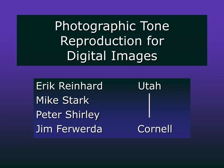
Photographic Tone Reproduction for Digital Images. Erik Reinhard Utah Mike Stark Peter Shirley Jim Ferwerda Cornell. Tone Reproduction Problem. Watch the light Compare with projection on screen. Overview. Tone reproduction is difficult when Dynamic range is high

E N D
Photographic Tone Reproduction for Digital Images Erik Reinhard Utah Mike Stark Peter Shirley Jim Ferwerda Cornell
Tone Reproduction Problem • Watch the light • Compare with projection on screen
Overview • Tone reproduction is difficult when • Dynamic range is high • Algorithm is used in predictive context • Requirements of a practical operator • Skip many details (see paper for those)
Dynamic Range • Ratio of brightest and darkest regions where detail is visible • Implies that some controlled burn-out is desirable! • Simplifies tone reproduction problem
Controlled Burn-out is OK No detail expected when looking into the sun (sunspots)
Zones Lin: 1 2 4 8 16 32 64 128 256 Log: 1 2 3 4 5 6 7 8 9 • Each doubling of intensity is new zone • Nine zones with visible detail can be mapped to print, fewer to displays • Zones are a good measure of dynamic range
Typical Dynamic Ranges • Photographs: 4-6 zones with visible detail (after digitizing) • HDR images: 7-11 zones with visible detail • Tone reproduction should not be very difficult for most images!
11 Zones 7 Zones
Rest of Talk: • A very simple global operator adequate for most images (up to 11 zones) • A local operator that handles very high dynamic range images (12 zones and more)
Global vs. Local • Global • Scale each pixel according to a fixed curve • Key issue: shape of curve • Local • Scale each pixel by a local average • Key issue: size of local neighborhood
Global Operator • Compression curve needs to • Bring everything within range • Leave dark areas alone • In other words • Asymptote at 1 • Derivative of 1 at 0
Global Operator Results 8 Zones 7 Zones
Global Operator Results 12 Zones
Global Operator Results 15 Zones
Local Operator • Replace • With • V1 is our dodge-and-burn operator
Dodge and Burn • Roughly equivalent to local adaptation • Compute by carefully choosing a local neighborhood for each pixel • Then take a local average of this neighborhood (which is V1)
Dodge and Burn Computation • Compute Gaussian blurred images at different scales (sizes) • Take difference of Gaussians to detect high contrast (Blommaert model) • Take Gaussian at largest scale that does not exceed contrast threshold (V1)
Subtleties • Gaussians computed at relatively small scales • For sufficient accuracy, computation rewritten in terms of the error function • For sufficient speed, computation performed in Fourier domain
Local Operator Results Light bulb visible Small halo around lamp shade Text on book visible 15 Zones
Conclusions • Most “high dynamic range” images are medium dynamic range • This makes tone reproduction a fairly straightforward problem for most practical applications/images
Conclusions • Our global operator is very simple and is adequate for most images • Our local operator is more involved and compresses very high dynamic range images adequately
Further Work • Two manual parameters: • Key value to determine overall intensity of result • White point to fix contrast loss for low to medium dynamic range images • Both can be automated with a straightforward algorithm – see forthcoming journal of graphics tools and my web page
Acknowledgments • Thanks to Greg Ward, Paul Debevec, Sumant Pattanaik, Jack Tumblin • This work was sponsored by NSF grants 97-96136, 97-31859, 98-18344, 99-78099 and by the DOE AVTC/VIEWS
Erratum Equation 1 in the paper should be: Note: source code on CDROM is correct!
Informal comparison Gradient-space[Fattal et al.] Bilateral[Durand et al.] Photographic[Reinhard et al.]
Informal comparison Gradient-space[Fattal et al.] Bilateral[Durand et al.] Photographic[Reinhard et al.]